the Creative Commons Attribution 4.0 License.
the Creative Commons Attribution 4.0 License.
 | 23 Oct 2019
Influence of multi-decadal land use, irrigation practices and climate on riparian corridors across the Upper Missouri River headwaters basin, Montana
Melanie K. Vanderhoof
Jay R. Christensen
Laurie C. Alexander
The Upper Missouri River headwaters (UMH) basin (36 400 km2) depends on its river corridors to support irrigated agriculture and world-class trout fisheries. We evaluated trends (1984–2016) in riparian wetness, an indicator of the riparian condition, in peak irrigation months (June, July and August) for 158 km2 of riparian area across the basin using the Landsat normalized difference wetness index (NDWI). We found that 8 of the 19 riparian reaches across the basin showed a significant drying trend over this period, including all three basin outlet reaches along the Jefferson, Madison and Gallatin rivers. The influence of upstream climate was quantified using per reach random forest regressions. Much of the interannual variability in the NDWI was explained by climate, especially by drought indices and annual precipitation, but the significant temporal drying trends persisted in the NDWI–climate model residuals, indicating that trends were not entirely attributable to climate. Over the same period we documented a basin-wide shift from 9 % of agriculture irrigated with center-pivot irrigation to 50 % irrigated with center-pivot irrigation. Riparian reaches with a drying trend had a greater increase in the total area with center-pivot irrigation (within reach and upstream from the reach) relative to riparian reaches without such a trend (p<0.05). The drying trend, however, did not extend to river discharge. Over the same period, stream gages (n=7) showed a positive correlation with riparian wetness (p<0.05) but no trend in summer river discharge, suggesting that riparian areas may be more sensitive to changes in irrigation return flows relative to river discharge. Identifying trends in riparian vegetation is a critical precursor for enhancing the resiliency of river systems and associated riparian corridors.


Riparian ecosystems provide critical biological, chemical and hydrological functions (Fritz et al., 2018). Defined as semi-terrestrial areas influenced by freshwaters at the interface of rivers and adjacent upland areas (Naiman et al., 2005), riparian ecosystems store water, nutrients and sediments, reducing downstream flood impacts and non-point source pollution (Lowrance et al., 1984; Vivoni et al., 2006). They also provide corridors for biotic movement and migration, particularly through arid, urban and agricultural landscapes (Boutin and Belanger, 2003; Lees and Peres, 2008), and maintain fish habitats by lowering stream temperatures and contributing in-stream woody debris (Poole and Berman, 2001; Isaak et al., 2012). Long-term trends in the degradation of riparian areas are common globally (Stromberg, 2001; Richardson et al., 2007). The hydrological alteration of rivers, including dam construction, drainage and water diversion ditches, flow regulation, and pumping of surface and groundwater for human use, can alter flow timing and magnitude, leading to riparian degradation including changes to riparian functioning, loss of riparian extent and shifts in species composition (Poff et al., 1997; Nilsson and Berggren, 2000; Sweeney et al., 2004). Periodic drought and continued water withdrawals degrade cold-water spawning and rearing habitats for salmonid species (Clancy, 1988; Isaak et al., 2012). Balancing anthropogenic water needs while maintaining or enhancing riparian ecosystem integrity requires an improved understanding of the relationship between water extraction, river discharge and riparian vegetation (Jones et al., 2010; Cunningham et al., 2011).
Irrigated agriculture is a primary consumptive use of water in the US and globally. Across the United States, 26 % of surface water withdrawals and 68 % of groundwater withdrawals are attributable to agricultural irrigation (Dieter et al., 2018). Globally, irrigation accounts for 70 % of water withdrawals (Wisser et al., 2008). Expansion of agricultural irrigation over the past centuries and shifts in irrigation methods over the past decades have led to major gains in agricultural productivity, food security, profitability and crop diversification (Falkenmark and Lannerstad, 2005). As a primary use of water withdrawals and water consumption, however, irrigated agriculture can be expected to play a key role in local water cycles. When gravity-fed (i.e., flood) irrigation is applied, water that is not evaporated or transpired by plants replenishes soil water storage, recharges aquifers, and contributes return flows to streams and wetlands (Peterson and Ding, 2005; Perry et al., 2017; Grafton et al., 2018). Additional groundwater recharge also comes from unlined ditch systems used to convey water to agricultural fields. Return flow from excess irrigation has been argued to have artificially elevated autumn and winter streamflow for decades (Kendy and Bredehoeft, 2006). As farmers switch to more modern irrigation techniques, such as center-pivot irrigation, they can achieve greater crop yields and gross revenue with less water, improving their “crop-per-drop” ratio (or water use efficiency; Peterson and Ding, 2005). This shift in irrigation practices, however, is expected to have hydrological consequences, namely increased evapotranspiration and a reduction in surface runoff and subsurface recharge (Ward and Pulido-Velazquez, 2008; Grafton et al., 2018) which can impact local aquifers (Peterson and Ding, 2005; Pfeiffer and Lin, 2014), base flow (Kendy and Bredehoeft, 2006; Gosnell et al., 2007) and potentially riparian ecosystems (Carrillo-Guerrero et al., 2013).
Water withdrawals for irrigation may impact local water cycling, but patterns in river discharge and riparian vegetation are largely driven by a watershed's climate patterns. Riparian vegetation tends to be adapted to highly variable fluvial disturbance regimes, a product of seasonal and interannual variability in river discharge, with riparian wetness peaking during episodic storm and flood events and lessening during drought events (Hughes et al., 2005; Goudie, 2006; Capon et al., 2013). River discharge and groundwater hydrology, in turn, tends to be highly responsive to variability in precipitation and evaporative demand (Goudie, 2006; Dragoni and Sukhiga, 2008; Hausner et al., 2018). Further, in snowmelt-dominated systems, changes in snowpack storage and rain to snow event ratios can influence the timing of river discharge and regional groundwater recharge, impacting water availability in associated riparian areas (Rood et al., 2008).
While satellite imagery offers a cost-effective means to monitor landscapes, the narrow, linear nature of riparian corridors presents a challenge for ecosystem characterization with remote-sensing tools (Klemas, 2014; Vanderhoof and Lane, 2019). Along large rivers, Landsat satellites provide a multi-decadal source of imagery to monitor changes in riparian vegetation (Jones et al., 2010; Henshaw et al., 2013). Remote sensing can also complement field data to enhance our understanding of the relationship between riparian vegetation and agents of change, such as climate (Huntington et al., 2016). The normalized difference vegetation index (NDVI; Tucker, 1979) is the most commonly used spectral index to evaluate changes in riparian vegetation over time (Fu and Burgher, 2015; Hamdan and Myint, 2015; Nguyen et al., 2015; Hausner et al., 2018). Trends in riparian greenness have been related successfully to climate variables and river discharge (Shafroth et al., 2002; Fu and Burgher, 2015; Nguyen et al., 2015), in part because riparian and wetland herbaceous species can respond rapidly to changes in soil moisture. Thus, riparian greenness tends to reflect river corridor hydrologic processes (Stromberg, 2001; Stromberg et al., 2006; Jones et al., 2008). Other indices can also potentially inform riparian wetness. For instance, the normalized difference wetness index (NDWI) was designed to be sensitive to changes in leaf and soil water content as well as to identify waters associated with wetlands or floodplains (Gao, 1996; McFeeters, 1996). This index has been used successfully, for example, to monitor changes in the extent of waterlogged areas (e.g., Chatterjee et al., 2005; Chowdary et al., 2008).
Despite the potential for satellite imagery to characterize plant–water interactions along riparian corridors, few studies have evaluated the impact of changing irrigation methods on riparian vegetation (Klemas, 2014; Perry et al., 2017) or have attempted to distinguish the relative influence of climate and agricultural irrigation on riparian vegetation. The Upper Missouri River headwaters (UMH) basin in southwestern Montana provides an excellent case study for exploring the interactions between climate, irrigation and riparian vegetation. The basin contains the Jefferson, Madison and Gallatin rivers, all of which support world-class cold-water trout fisheries that provide substantial economic value to the region (Duffield et al., 1992; Kerkvliet et al., 2002; Gosnell et al., 2007). In addition, the agricultural valleys of the basin are very productive yet rely on a complex irrigation system to water crops grown in and near riparian areas. Irrigation accounts for 97 % of Montana's consumptive water use (Clifford, 1995; Dieter et al., 2018). Along with the high demand for irrigation water (Goklany, 2002; Schaible and Aillery, 2012), there are also increasing public water supply needs in the basin (Hansen et al., 2002; Gude et al., 2006). Finally, the timing of peak river flows is predicted to change, attributable to warmer temperatures at higher elevations and more precipitation in winter and early spring occurring as rainfall rather than snow (Pederson et al., 2011, 2013; USBR, 2012). All these factors contribute to an increasingly uncertain supply of water across the basin, particularly in the late summer. This uncertainty, in turn, has elevated interest in improving the resiliency of local streams and rivers so that the basin can continue to support the agricultural, recreational, municipal and ecological needs of the watershed (Montana DNRC, 2014, 2015; Montana Drought Demonstration Partners, 2015; McEvoy et al., 2018). In this study we used a time series of Landsat imagery (1984–2016) together with climate datasets, agricultural datasets and US Geological Survey (USGS) stream gage datasets to explore trends over time in riparian vegetation for the major river valleys across the UMH basin. We sought to link the temporal trends not explained by climate to changes in land use type and intensity. Our research questions were as follows:
-
How does remotely sensed riparian wetness across the UMH basin reflect interannual variability in climate and river discharge?
-
How and to what degree are trends in riparian wetness from 1984 to 2016 attributable to changes in climate versus shifts in land use such as irrigation practice?
2.1 Study area
The study area was the UMH basin (36 400 km2). Near the basin outlet, the Jefferson, Madison and Gallatin rivers merge to form the Missouri River at Three Forks, Montana. A total of nine rivers were included in the analysis, with riparian vegetation divided into 19 riparian reaches (Fig. 1). Hydrologic regimes of the rivers across the basin are snowmelt dominated (Markstrom et al., 2016; Cross et al., 2017), with multiple mountain ranges contributing surface runoff and groundwater recharge to valley aquifers (Hackett et al., 1960; Slagle, 1995). Annual precipitation across the basin averages 565 mm yr−1, most of which falls in the mountains, where it is received primarily as snow (Fig. 2). The annual maximum and minimum temperatures average 10 and −3 ∘C, respectively (1981–2010 period of record; PRISM Climate Group, 2018). Elevations across the basin range from 1231 to 3433 m (Gesch et al., 2002). While the mountain ranges are dominated by evergreen forest (35 %), at lower elevations, the forest gives way to herbaceous vegetation (35 %) and shrub or scrub (20 %) cover types that dominate the large river valleys (Homer et al., 2015; Fig. 2). Agriculture occurs primarily in the lower elevations adjacent to many of the major rivers. As of 2017, alfalfa was the most common crop (41 %), followed by other non-alfalfa hay crops (25 %), barley (11 %) and spring wheat (11 %; USDA, 2018). The riparian ecosystems along the major rivers are dominated by tree species including cottonwood (Populus spp.), willow (Salix spp.) and alder (Alnus spp.); shrubs including chokecherry (Prunus virginiana), snowberry (Symphoricarpos spp.) and wild rose (Rosa woodsia); and wet meadows dominated by cattails (Typha spp.), sedges (Carex spp.) and rushes (Juncus spp.). Warming temperatures in March and April initiate snowmelt and a corresponding increase in river discharge. Spring precipitation and snowmelt produce peak river discharge in May and June (Cross et al., 2017), followed by a sharp decline in July and August due to a dwindling supply of meltwater from snowpack and consumptive use from withdrawals. Late autumn through early spring is generally characterized by lower-flow conditions, presumably dominated by baseflow contributions from groundwater discharge (Cross et al., 2017). Major waterbodies across the basin are predominately reservoirs located upstream from dams (Fig. 1b) that support irrigation, hydropower and recreation.
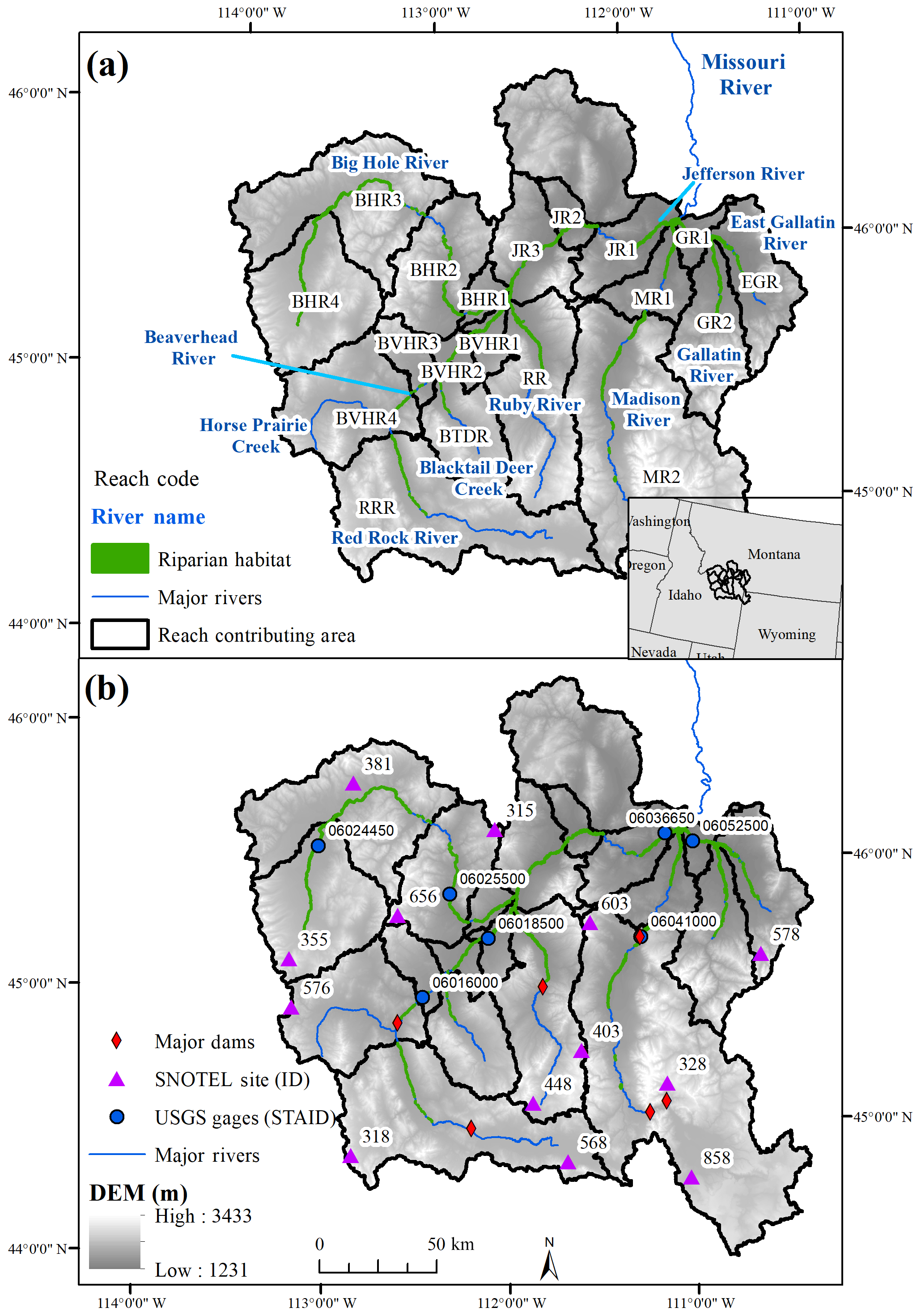
Figure 1(a) The major rivers considered in the analysis, the distribution of the riparian areas evaluated, and the division of the riparian areas into reaches across the Upper Missouri River headwaters basin, southwestern Montana, USA. (b) The spatial distribution of the US Geological Survey stream gages and snow telemetry (SNOTEL) sites considered in the analysis. STAID: station ID. DEM: digital elevation model.
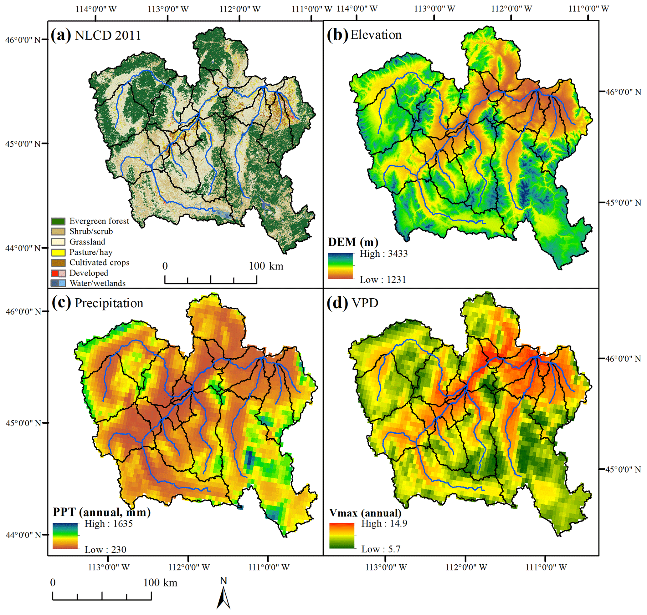
Figure 2Spatial variability in (a) land cover, defined using the 2011 National Land Cover Database (NLCD), (b) elevation, (c) mean annual precipitation (PPT) and (d) mean annual vapor pressure deficit (VPD) across the Upper Missouri River headwaters basin. DEM: digital elevation model. Vmax: maximum vapor pressure deficit.
2.2 Unit of analysis
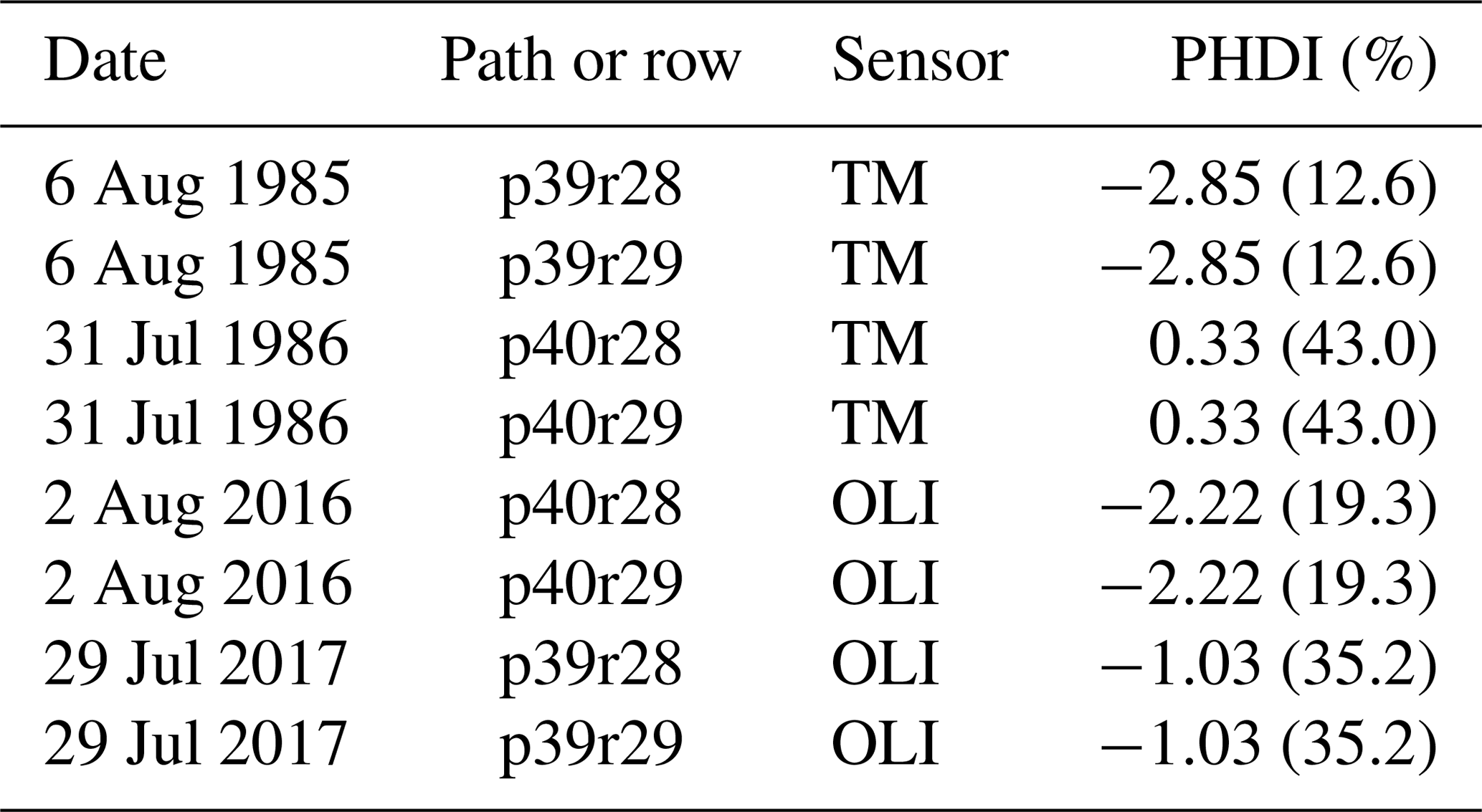
The objective of this study was not to document changes in the total amount of riparian vegetation but instead to document temporal variability and trends in the wetness of persistent riparian vegetation in relation to climate and landscape variables. The extent of persistent riparian vegetation in major river valleys was delineated manually using Landsat imagery from 1985, 1986, 2016 and 2017 (Table 1). National Agricultural Imaging Program (NAIP) imagery was also used to improve accuracy in areas where agriculture was inter-mixed with riparian vegetation. The active river channel was excluded from the area of analyses. For headwater reaches, riparian areas upstream of all identifiable irrigated agriculture were excluded from the analysis. This approach enabled us to reduce uncertainty in the vegetation types and the temporal analysis but potentially limited our ability to include changes where there was a complete loss or novel gain of riparian vegetation.
Table 1Landsat images used to map agricultural extent. The Palmer hydrological drought index (PHDI) values were provided for the month of July. The percentage was calculated based on the values that occurred between 1984 and 2017. TM: thematic mapper. OLI: operational land imager.
For trend analysis, we used river topology, topography and clusters of irrigated agriculture to divide the delineated riparian areas into 19 study reaches (Table 2; Fig. 2). After riparian reach lengths were defined, the per reach contributing area was calculated using the Spatial Tools for the Analysis of River Systems (STARS, v 2.0.4; Peterson, 2017). All pits and flow interruptions in the digital elevation model (DEM) were filled. The flow direction for the river network was generated, and the rivers burned into the DEM. The area contributing to the downstream point of each riparian reach (n=19) was estimated so that each contributing area was non-overlapping with edge-matching inter-basins (Theobald et al., 2006; Table 2; Fig. 1).
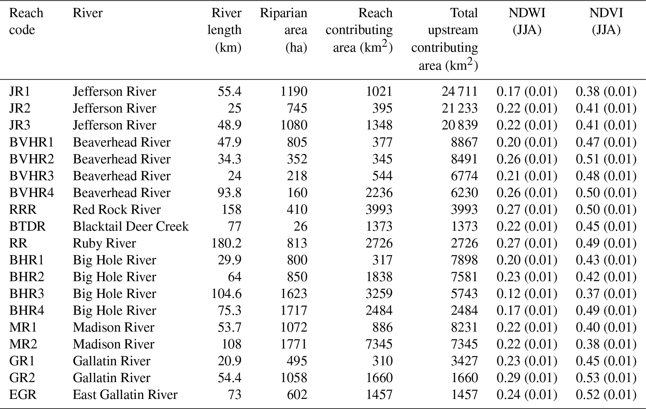
Table 2Characteristics of each riparian reach considered, including river length, riparian area analyzed, riparian reach contributing area and average (1984–2016) growing-season (June, July and August – JJA) normalized difference wetness index (NDWI) and normalized difference vegetation index (NDVI). Standard error shown in parentheses.
2.3 Dependent variable
The NDWI calculated from Landsat imagery (NIR − SWIR1)∕(NIR + SWIR1; Gao, 1996; McFeeters, 1996) was used to estimate riparian wetness. Relative to other indices such as the NDVI, the NDWI is considered to be less sensitive to atmospheric conditions, including the solar elevation angle, sensor angle and atmospheric conditions, making it suitable for time-series analysis (Crétaux et al., 2015), and has been used to monitor patterns in waterlogged areas (e.g., Chatterjee et al., 2005; Chowdary et al., 2008). Reach-scale average NDVI and NDWI values were provided to give a sense of the reach-scale variability in spectral characteristics (Table 2). NDWI values greater than approximately 0.3 are typically used to distinguish open water (Chatterjee et al., 2005; Chowdary et al., 2008; McFeeters, 2013). Across the UMH basin, we determined that riparian NDWI values were more sensitive to interannual variability in climate (Fig. 3) and river discharge than the NDVI, making it a more appropriate index for this analysis. Per year, average NDWI values (June–August 1984–2017; 102 values per riparian reach) were calculated using the Landsat surface reflectance image collections in Google Earth Engine for all delineated riparian reaches (n=19). June, July and August were selected to correspond to peak months for irrigation water withdrawals (Bauder, 2018). Potentially erroneous values were defined as values that were greater or less than ±2 standard deviations from the riparian reach-specific monthly mean and were removed. To normalize the data for seasonality, values were calculated as the anomaly from the riparian reach-specific, long-term (1984–2017) mean monthly value (NDWI anomaly). The monthly (June–August) anomaly values were then averaged per year to provide a single NDWI anomaly per summer per reach. The multi-month approach compensated for data gaps created when cloud cover masked Landsat NDWI values.

Figure 3A visual comparison of index values in a dry year (2001; 431 mm annual precipitation) and a wet year (1995; 687 mm annual precipitation) at the confluence of Jefferson, Madison and Gallatin rivers. The normalized difference wetness index (NDWI) in the riparian vegetation showed more variability in response to precipitation relative to the normalized difference vegetation index (NDVI). A comparison of (a) NDVI (July 2001), (b) NDWI (July 2001), (c) raw Landsat image (1 July 2001), (d) NDVI (July 1995), (e) NDWI (July 1995) and (f) raw Landsat image (17 July 1995). A similar pattern was observed across the basin.
2.4 Independent variables
Climate variables derived from the Parameter-elevation Regressions on Independent Slopes Model (PRISM; 4 km resolution; PRISM Climate Group, 2018) included annual precipitation, annual lagged (1 year) precipitation, winter precipitation (January–March), spring precipitation (March–May), summer precipitation (June–August), spring maximum and minimum temperature (March–May), summer maximum and minimum temperature (June–August), and maximum vapor pressure deficit (VPD; spring and summer). VPD represents a measure of the drying power of the air and is a function of air temperature and humidity. Across the contributing area of each riparian reach (n=19), 100 points were randomly selected (total points = 1900). To generate basin-wide values, the climate values for each year (1984–2016) were extracted for each point, averaged for the reach and then weighted using the relative size (ha) of each reach across the basin. Because upstream climate, such as snowfall or precipitation, can influence downstream riparian wetness, climate variables for each riparian reach were similarly calculated using the area-weighted average values for that reach and all reaches contributing to that reach.
To characterize interannual variability in snowfall, we used a total of 13 Snow Telemetry (SNOTEL) sites (IDs: 315, 318, 328, 355, 381, 403, 448, 568, 576, 578, 603, 656 and 858). Annual total snowfall (September–August) and total spring snowfall (March–July) were calculated for each SNOTEL site. For each riparian reach we identified the nearest one or two SNOTEL sites, using the SNOTEL site immediately upstream from the riparian reach as available. When two SNOTEL sites were used, the snowfall amounts were averaged across the two sites. Only sites with data available for the entire period of 1984–2017 were used (NSIDC, 2018). To further characterize climate conditions, we included the monthly Palmer drought severity index (PDSI) and the Palmer Z index for NOAA NCDC Division 2 in Montana. Both indices are calculated from precipitation and temperature station data and interpolated at 5 km (NOAA NCDC, 2014). The PDSI represents the accumulation or deficit of water over approximately the past 9 months, while the Palmer Z index represents the current monthly conditions with no memory of previous deficits or surpluses (NOAA NCDC, 2014). The indices were averaged to spring (March–May), summer (June–August) and the whole year and represent multi-month averages of the drought indices. Temporal trends (1984–2016) in the climate variables were tested at the basin scale using the non-parametric Mann–Kendall test for trends (Kendall R package; Mann, 1945; Kendall, 1975; Gilbert, 1987). Each SNOTEL site was tested independently for temporal trends in snowfall.
2.5 Agricultural patterns
We sought to relate patterns in riparian wetness to patterns in total irrigated agricultural area and the relative abundance of irrigation methods. Existing sources of data, such as the Montana Department of Revenue's Final Land Unit (FLU) Classification (2010 and 2017) or the USGS (county-scale) Water Use Surveys (1950–2015), lacked a spatially explicit dataset of agricultural extent and irrigation methods for the early part of the Landsat archive (1980s). Therefore, we generated two agricultural extent datasets representing the two temporal ends of the Landsat archive (1985–1986 and 2016–2017). The Landsat images used to define the active cropland extent are shown in Table 1. Cloud cover was only present in the mountainous areas in all images used. We recognize that by using a single Landsat image (instead of multiple images collected over the growing season) and only representing the ends of the study time span, we may be underestimating agricultural extent and missing year-to-year variability in agricultural activities. Generating agriculture extent and irrigation types for the beginning and end of our study period, however, enabled us to identify spatially explicit trends or shifts in agricultural practices that have been previously shown at a county or state scale (USDA, 2018). Cropland extent was generated initially using eCognition 9.2 software (Trimble, Westminster, CO). The Landsat images were segmented into objects using the near-infrared (NIR), red and green bands. The FLU 2017 data layer was used to mask out non-crop and non-pasture land cover types. The objects were classified as agriculture or non-agriculture using NDVI thresholds. The draft agricultural outputs were then manually edited to add and remove agricultural fields as needed. Fallow fields were not included in the agricultural extent, as they were assumed to be non-irrigated for that year. For overlapping portions between adjacent Landsat images, a field was included as crop if it was identified as such in either image. It is possible there could be potential confusion between non-center-pivot irrigation and non-irrigated fields; however, 92 % and 93 % of the 1985–1986 and 2016–2017 agricultural area, respectively, co-occurred with Montana FLU polygons classified as irrigated, suggesting that non-irrigated agriculture is a minority cover class across the UMH basin.
Active crop fields were further classified manually as center-pivot irrigation or non-center-pivot irrigation (e.g., gravity-fed, non-center-pivot sprinklers such as tower sprinklers, solid set and permanent sprinklers, side roll, big gun or traveler sprinklers, or hand-move sprinklers) based on field shape (i.e., round or not round). For reference, the FLU polygons were classified as center pivot, sprinkler or gravity-fed using irrigation infrastructure (gates, ditches and dikes) identifiable from NAIP images (1 m resolution). Sprinkler irrigation was distinguished using parallel wheel lines. Because this irrigation infrastructure was not visible in the Landsat imagery, we did not attempt to distinguish gravity-fed irrigation from non-center-pivot sprinkler irrigation. Consequently, the datasets as created enabled us to quantify changes in irrigation extent and any shifts in center-pivot irrigation. It did not allow us to make estimates of water consumption or quantify shifts from gravity-fed irrigation to non-center-pivot sprinkler irrigation.
2.6 Analysis
Temporal trends in riparian wetness (NDWI anomaly) were tested for each riparian reach using the non-parametric Mann–Kendall (MK) test for trends. As the MK test for trends can be sensitive to temporal autocorrelation (Hamed and Rao, 1998), we used the Durbin–Watson statistic to test for the presence of temporal autocorrelation in the NDWI anomaly values of each riparian reach. Because autocorrelation can inflate trend significance, in reaches where temporal autocorrelation was present, we calculated a modified Mann–Kendall test for trends that accounts for the autocorrelation structure of the data (Hamed and Rao, 1998).
Interannual variability in riparian wetness for a given reach can be expected to be a function of (1) interannual climate variability and (2) changes in the amount and timing of anthropogenic water withdrawals or water return flow, while spatial variability in these relationships can be expected to be a function of landscape characteristics. Temporal variability in climate and anthropogenic activities could occur both within each reach and upstream of each reach. Because annual (1984–2016) agricultural and irrigation data were not available for the entire time series, the influence of water withdrawals was estimated as the residual variance after modeling the interannual variability in riparian wetness attributable to climate.
The NDWI anomaly values were related to climate variables for each riparian reach using random forest analysis. The random forest analyses were used to quantify the amount of variation in the NDWI anomalies explained by climate variables and to identify the frequency (importance) of specific climate variables in predicting NDWI anomalies. Random forest techniques use bootstrapping to employ hundreds of regression trees and make no prior assumptions about cause and effect relationships or correlations among variables (Hastie et al., 2009). Random forest techniques are generally insensitive to multicollinearity; however, the inclusion of highly correlated variables can deflate both variable importance and the overall variation explained by the analysis, while the inclusion of many variables can make interpretation difficult and introduce noise (Murphy et al., 2010). We therefore implemented variable selection using the rfUtilities package in R (Murphy et al., 2010) before running random forest regressions for each riparian reach with the selected subset of climate variables. To model growing-season riparian NDWI anomalies we calculated 500 regression trees for each riparian reach. We did not restrict the number of nodes; model overfit was instead limited by setting the minimum sample size per node to 5. Because of the limited data points per riparian reach (n=33) model fit was assessed using out-of-bag (OOB) root-mean-squared error (RMSE; 70 % of points used to train, 30 % of points used to validate) using the randomForest package in the R statistical software (Liaw and Wiener, 2015). We found no increase in the OOB error as more trees were generated (i.e., up to 500 trees). Random forest regression residuals were then extracted and evaluated for temporal trends not attributable to climate variability. Temporal trends in the regression residuals were tested using the non-parametric MK test for trends. We again used the Durbin–Watson statistic to test for the presence of temporal autocorrelation in the NDWI anomaly–climate regression residual values of each riparian reach. If temporal autocorrelation was significant, the modified Mann–Kendall test for trends was used instead.
We note that we tested an alternative method in which data for all riparian reaches and years were combined in a single linear mixed model. This approach increased our sample size (33 years × 19 riparian reaches), but we found that the error in the regression, specifically the strength of the relationship between the predicted and actual NDWI anomalies, was uneven between riparian reaches, thereby decreasing our confidence in the analysis of trends in the residuals. This finding further supported our decision to run a random forest regression for each riparian reach.
2.7 Ancillary spatial datasets
Landscape characteristics such as topography, geology and land cover may influence how riparian vegetation responds to climate variability over time and were therefore also considered. Between-group differences in landscape characteristics were calculated for riparian reaches that showed a temporal trend in riparian wetness relative to riparian reaches that showed no temporal trend in riparian wetness using the non-parametric Mann–Whitney–Wilcoxon test (or the Wilcoxon rank sum test; Cohen, 1988). Variability in topography was quantified as the (1) elevation coefficient of variation across each 10-digit hydrologic unit code (HUC10; Ascione et al., 2008) as well as the (2) Melton ruggedness number, which is calculated as the maximum elevation minus the minimum elevation divided by the area of the hydrological unit (HUC10; Melton, 1965), using the USGS National Elevation Dataset (NED) 10 m resolution (Gesch et al., 2002). The percentage of the riparian reach's within reach contributing area that was (1) evergreen forest, (2) herbaceous vegetation, (3) pasture and (4) crop was included, as classified by the National Land Cover Database (NLCD) 2011 (Homer et al., 2015). Soil and geology characteristics were considered using the minimum water table depth (April–July), bedrock depth and soil drainage characteristics, specifically the percentage of each riparian reach's contributing area that is well drained (excessively drained, somewhat excessively drained or well drained) and poorly drained (very poorly drained or poorly drained). These variables were derived from the National Resources Conservation Service's Soil Survey Geographic (SSURGO) Database to characterize infiltration capacity (Soil Survey Staff, 2018). Change in developed (built-up) land, including urban, residential and commercial land uses, was quantified using the “Historical built-up intensity layer (1810–2015, 5-year intervals)” (Leyk and Uhl, 2018). This dataset quantifies the sum of building areas of all structures per pixel, where pixel size is 250 m by 250 m. Change in built-up intensity was quantified as the change in the sum of building areas between 2015 and 1985 (m2) per river length (m).
2.8 River discharge
Riparian corridors are interconnected with its adjacent rivers via longitudinal, lateral and vertical fluxes of water (Fritz et al., 2018). To explore the potential relationship between riparian water storage and river discharge across the UMH basin, we identified seven USGS stream gages within the basin, with upstream contributing areas ranging between ∼3400 and ∼25 000 ha. The gages were variable in their position relative to flow regulators such as dams associated with lakes or reservoirs. The amount of flow regulation enforced by these flow regulators was unknown and therefore a major point of uncertainty. The Spearman correlation coefficient was calculated between the monthly river discharge, averaged to June–August, and the riparian NDWI anomalies for the co-located riparian reach or the riparian reach immediately adjacent to each gage. We note that a correlation can be indicative of a similar response of both variables to interannual water availability (e.g., precipitation) as well as potential movement of water across the river–upland interface. We also evaluated trends in river discharge over time (1984–2016) in the growing season (June, July and August) as well as autumn (September, October and November) and winter (December, January and February) seasons using the MK test for trends. The temporal trends in river discharge were calculated only to compare with temporal trends in riparian wetness over the same period. We note that a full trend analysis in river discharge would require not only utilizing the entire record of river discharge available per gage but also considering the potential impact of flow regulation via dams as well as interannual variability in surface withdrawals for irrigation, which are closely regulated by Montana state law (Montana DNRC, 2015).
3.1 Trends in riparian wetness
A total of 15 785 ha (157.85 km2) of riparian vegetation was delineated along the major rivers (Fig. 1). River length within each riparian reach ranged from 21 km along the Gallatin River to 180 km along the Ruby River and averaged 70 km in length (Table 2; Fig. 1). The total riparian area analyzed per reach ranged from 26 ha (289 Landsat pixels) along the Blacktail Deer Creek to 1771 ha (19 678 Landsat pixels) along the Madison River and averaged 831 ha (9233 Landsat pixels; Table 2). The NDVI and NDWI averaged 0.45 and 0.22, respectively, across riparian reaches and years (Table 2). All 19 riparian reaches showed an average NDWI of <0.3 (Table 2), the threshold that is typically used to identify open water (Chatterjee et al., 2005; Chowdary et al., 2008; McFeeters, 2013). Temporal autocorrelation was found to be significant for the NDWI anomaly data over time in 3 of the 19 riparian reaches, but in all three cases, the autoregressive model (AR1) performed worse than the linear model, as evaluated by comparing Akaike information criterion (AIC) values (Hurvich and Tsai, 1989), suggesting that autoregressive models were not appropriate for this analysis (Table 3). For these three reaches, and three reaches for which the residuals were found to show temporal autocorrelation, the modified MK test for trends was used.
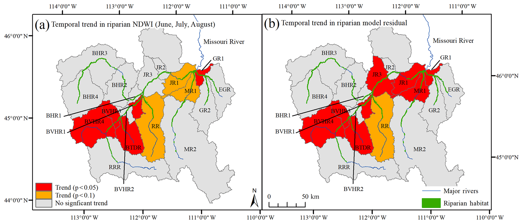
Figure 4(a) The spatial distribution of riparian reaches found to show a significant decreasing trend (p<0.1 or p<0.05) in riparian wetness using the normalized difference wetness index (NDWI; June, July and August) anomalies, and (b) the spatial distribution of riparian reaches found to show a significant trend in NDWI anomaly–climate regression residuals or the variance in NDWI anomalies not explained by climate variables. All trends were negative, indicating a drying over time.
Table 3Temporal trends in per reach riparian normalized difference wetness index (NDWI; June, July and August) anomalies using the Mann–Kendall (MK) test for trends. The Durbin–Watson (DW) statistic was used to test for the presence of temporal autocorrelation. NDWI anomalies were modeled against climate variables using random forest regressions. The temporal trends in the random forest regression residuals were evaluated using MK test for trends. A modification of the MK (Hamed and Rao, 1998) was used for the reaches where the DW statistic was significant. RMSE: root mean square error. *: p<0.1. : p<0.05.
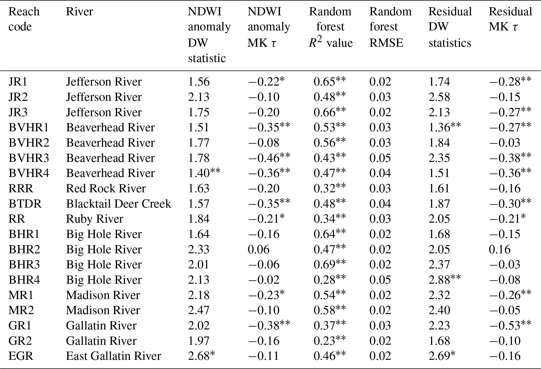
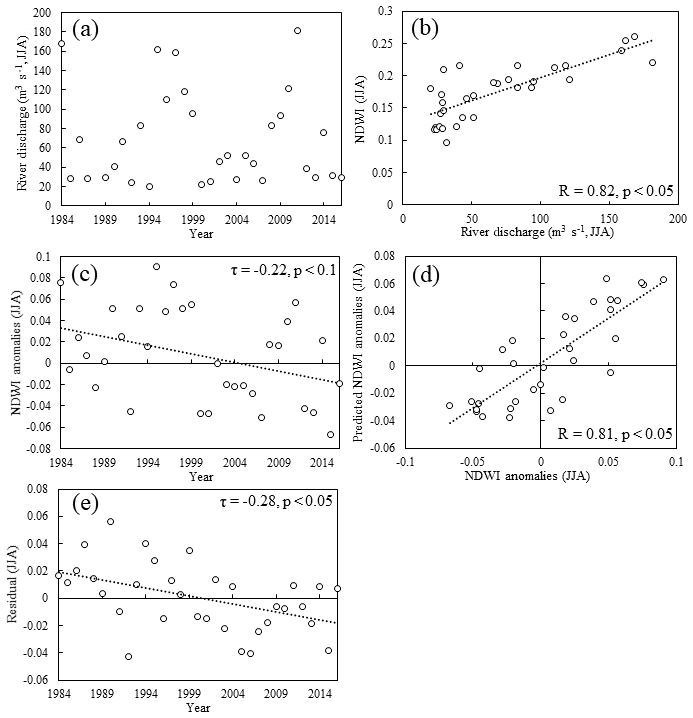
Figure 5Statistics for the Jefferson River riparian reach at the basin outlet (JR1), including (a) variability in June, July and August (JJA) river discharge over time (station ID: 6036650); (b) relationship between the normalized difference wetness Index (NDWI) and river discharge; (c) trend in NDWI anomalies over time; (d) correlation between NDWI anomalies and predicted NDWI anomalies; and (e) trend in NDWI anomaly–climate regression residuals over time.

Figure 6Statistics for the Gallatin River riparian reach downstream of the East Gallatin River (GR1), including (a) variability in river discharge over time (station ID: 6052500), (b) relationship between the normalized difference wetness index (NDWI) and river discharge, (c) trend in NDWI anomalies over time, (d) correlation between NDWI anomalies and predicted NDWI anomalies, and (e) trend in NDWI anomaly–climate regression residuals over time.
When we tested for MK trends in growing-season (June–August) riparian wetness over time, 8 of the 19 riparian reaches showed a significant decline over time in growing-season NDWI anomalies (five riparian reaches p<0.05; three riparian reaches p<0.1; Table 3; Fig. 4). The BVHR3 and BVHR4 riparian reaches that tested positive for autocorrelation still showed a significant drying trend after using the modified MK test. Interannual variability in climate can be expected to explain a portion of the interannual variability in riparian wetness. Across all 19 reaches, climate variables explained 23 % to 69 % (averaged 47 %) of the interannual variability in riparian NDWI anomalies (Table 3). However, basin-wide, the climate variables did not show a temporal trend over same period (1984–2016), apart from the VPD maximum (summer), which showed an increasing trend (p<0.1; Table 4). Drought indices, in particular the PDSI (summer, selected in 15 regressions, and annual, selected in 13 regressions) but also the Palmer Z index (annual and spring both selected in nine regressions) as well as annual precipitation (selected in 11 regressions) were the variables most frequently selected for inclusion in the random forest analyses (Table 4).
For the eight riparian reaches that showed a temporal trend in NDWI anomalies (Fig. 4a) the NDWI anomaly–climate regression residuals also showed a significant negative trend over time, indicating that declines in riparian wetness cannot be attributed solely to climate variability (seven riparian reaches p<0.05; one riparian reach p<0.1; Table 3; Fig. 4b). One additional riparian reach along the Jefferson River (JR3) did not show a significant trend in NDWI anomalies but did show a significant negative trend in the NDWI anomaly–climate regression residuals (p<0.05, Table 3; Fig. 4). The riparian reach BVHR1 also showed a significant negative trend in the NDWI anomaly–climate regression residuals when tested using the modified MK test. Data for two of the riparian reaches at the basin outlet (JR1 and GR1) are shown in Figs. 5 and 6, respectively. Both show a decline in NDWI anomalies over time, with the slope of the relationship steepening after the removal of the climate component (Figs. 5 and 6).
3.2 Trends in agriculture and water withdrawals
Agriculture across the UMH basin is spatially distributed along the major rivers (Fig. 2a). Using the endpoint (1985–1986 and 2016–2017) agriculture dataset, the largest amounts of agriculture occurred along the Gallatin River, Beaverhead River, Ruby River and the most upstream reach of the Big Hole River (Fig. 7a). The effect of water withdrawals can be expected to accumulate downstream; therefore the total in hectares of upstream agriculture was highest along the Beaverhead River, Jefferson River and downstream portion of the Gallatin River (Fig. 7b).

Figure 7Changes in agricultural and development characteristics across Upper Missouri River headwaters basin between 1985–1986 and 2016–2017, including (a) total per reach agriculture (2016–2017), (b) total agriculture within and upstream of each reach (i.e., accumulated agriculture; 2016–2017), (c) change in the extent of center-pivot irrigation (1985–1986 to 2016–2017), (d) change in the extent of non-pivot irrigation (1985–1986 to 2016–2017), (e) change in total per reach agriculture (1985–1986 to 2016–2017), and (f) change in built-up intensity, defined as the summed building area at 250 m resolution (1985 to 2015).
Over the study period the total hectares of land in active agricultural production increased by 10.5 % (Table 5). The largest increases in total hectares were observed along the Gallatin and Jefferson rivers, while minor declines in total hectares were observed across the most upstream portion of the basin (Figs. 7 and 8). We also observed changes in irrigation methods. The basin-wide area irrigated using center pivot increased from 8961 ha (9 % of irrigated area) to 54 295 ha (50 % of irrigated area), while non-center pivot (gravity, non-center-pivot sprinklers) decreased from 89 049 ha (91 % of irrigated area) to 54 009 ha (50 % of irrigated area; Table 5). Aerial imagery shows examples of the conversion to center-pivot irrigation between 1985 and 2017 (Fig. 8). The percentage change in the proportion of agricultural land area using center-pivot irrigation ranged from 0 % to +58 % across the reaches, with the biggest conversions along the Jefferson, Beaverhead, Madison and Blacktail Deer rivers (Table 5).
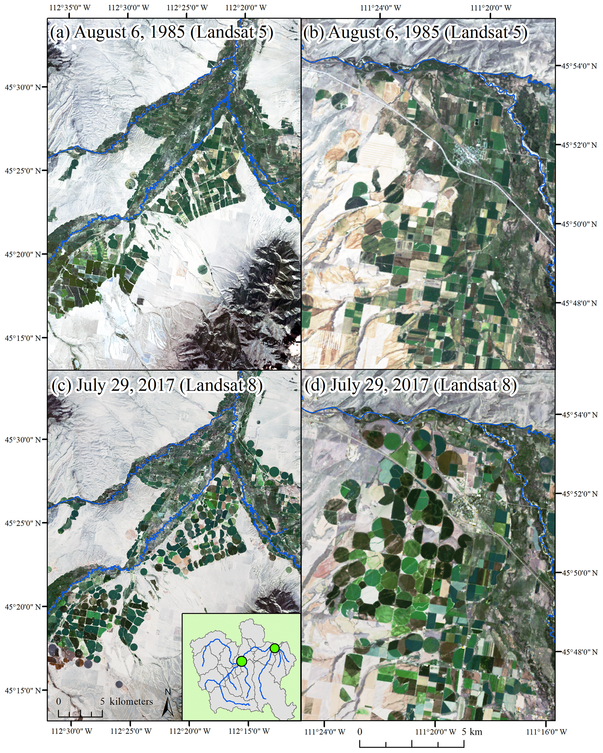
Figure 8Examples of areas showing a shift in irrigation technique over the past 30 years across the Upper Missouri River headwaters basin, including examples at the confluence of the Beaverhead (center), Big Hole (left) and Ruby River (right), shown in (a) and (c), as well as examples along Gallatin River, shown in (b) and (d).
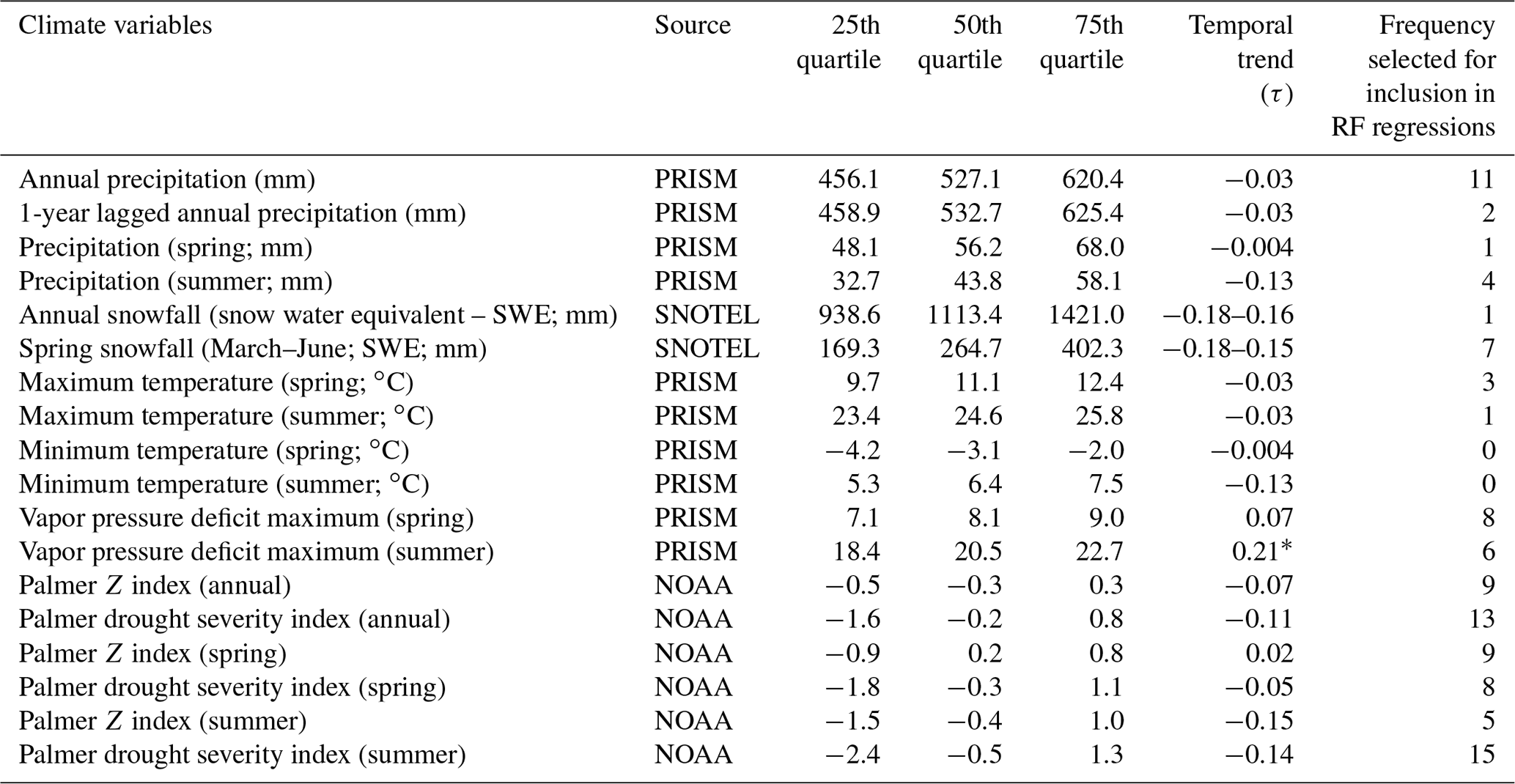
Table 4Climate variables considered in the analysis to represent interannual variability in conditions. The 25th, 50th and 75th quartile are shown to indicate the variability in the per riparian reach values included in the random forest (RF) regressions (n=19). The frequency of variable selection for inclusion in the random forest regressions is also shown. When tested at a basin scale for the time period of 1984–2016, no climate variables showed a significant temporal trend except the summer vapor pressure deficit (). PRISM: Parameter-elevation Regressions on Independent Slopes Model. SNOTEL: snow telemetry. NOAA: National Oceanic and Atmospheric Administration. Summer: June, July and August. Spring: March, April and May.
The conversion of irrigation methods could help explain the drying trends. Riparian reaches that saw a significant decline in riparian wetness, even after accounting for variability explained by climate, and showed several differences relative to riparian reaches where no such temporal trend was observed. First these drying reaches showed a greater average increase (within and upstream from the reach) in center-pivot irrigation area (+11 459 ha on average relative to +5634 ha) over the period (Mann–Whitney–Wilcoxon; p<0.05; Table 5). These reaches also showed a greater reach-scale change in the fraction center-pivot irrigation (+46 % average relative to +32 %; p<0.1) as well as a greater change in the fraction of center-pivot irrigation across a reach's contributing area (42 % average relative to 27 %; p<0.1; Table 5).
The response of a riparian reach to changes in water withdrawals and irrigation method may also depend on other landscape characteristics such as soil, geology and topography. Riparian reaches that showed a significant non-climate-related drying over time showed a higher percentage of well-drained soils (p<0.05) and a higher Melton ruggedness number (greater range in elevation per area; p<0.05; Table 6). In addition, although irrigation dominates water consumption across the basin, we note that development has increased around Bozeman, along the East Gallatin River, over the study period, while minimal increases in development were found elsewhere (Fig. 7f).
Table 5The per reach abundance of irrigated agriculture (Ir) at the two ends of the time period considered (1985–1986 and 2016–2017). Irrigation method was identified as center-pivot agriculture or non-center-pivot agriculture based on field shape. Accumulated (accum.) agriculture is defined as the summed area of agriculture across the total contributing area of each reach (e.g., GR1 is agriculture area in GR1, GR2 and EGR). Riparian reaches that showed a significant non-climate-related drying over time are shaded in gray. 1: headwater reach. *: p<0.1. : p<0.05.

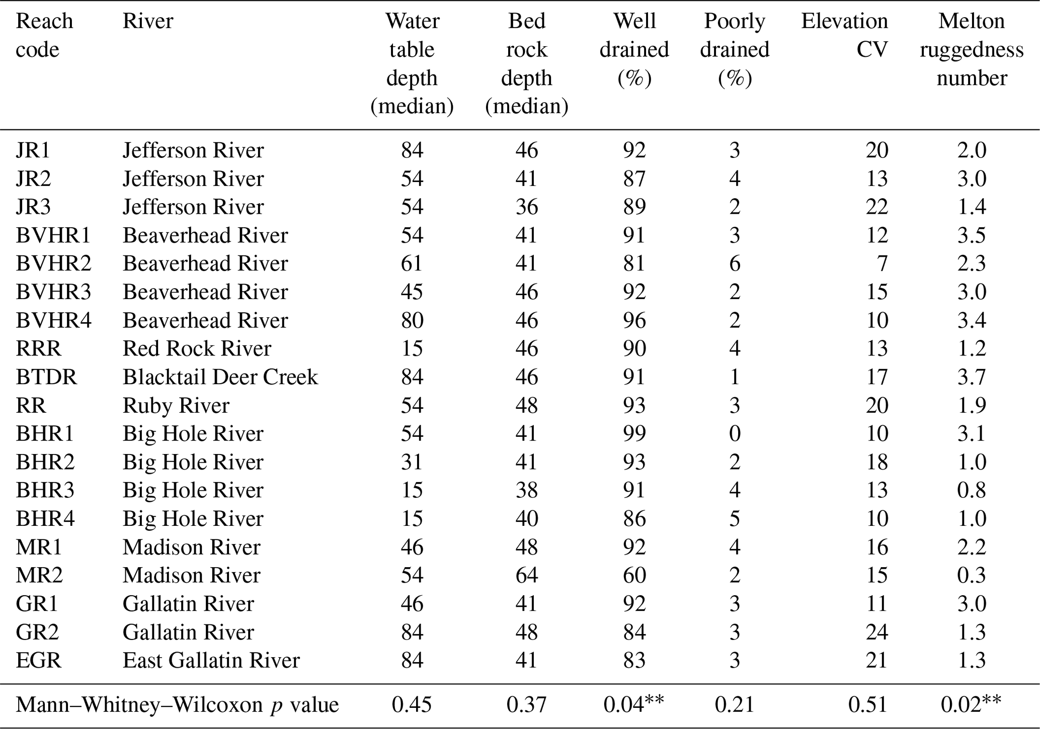
Table 6Characteristics of riparian reach contributing areas, including median water table depth (m), median bedrock depth (m), percentage of well-drained (or very well drained) soil, percentage of poorly (or very poorly) drained soil, elevation coefficient of variation (CV) and Melton ruggedness number. The Mann–Whitney–Wilcoxon test was used to calculate a measure of the difference (or lack of) between riparian reaches that showed a significant non-climate-related drying over time (shaded gray) and riparian reaches that showed no such pattern, with two asterisks indicating a significant difference (p<0.05) between the two groups.
The examples in Figs. 5 and 6 fit the pattern of a shift towards center-pivot irrigation and a corresponding drying trend in riparian wetness. Other reaches, however, showed less intuitive patterns. For instance, all reaches that showed a significant drying trend also showed a substantial increase in the fraction of center-pivot agriculture, ranging from 35 % to 64 %, except BVHR4, which showed a significant drying trend without an associated increase in center-pivot agriculture (a 24 % increase in center-pivot agriculture but the lowest total hectares of center-pivot irrigation in 2016–2017 of any riparian reach). The NDWI anomalies and NDWI anomaly–climate residuals shown in Fig. 9a and b indicate that this stretch of the Beaverhead River (BVHR4), which is immediately downstream from the Clark Canyon Reservoir, experienced a steep decrease in riparian wetness in 2002, with no visible trend before or after 2002. Such a clear steep decrease, however, was not observed in the closest stream gage (station ID: 06016000) downstream of this riparian reach. In contrast, one riparian reach on the Beaverhead River further downstream (BVHR2) showed a 54 % increase in the fraction of center-pivot agriculture as well as a decrease in the total hectares of irrigated agriculture over the study period (−48.5 ha km−1 river length), with no drying trend (Fig. 9c and d), even though reaches upstream and downstream of BVHR2 show significant drying trends. With the landscape characteristics considered we were again unable to determine why this riparian reach was more resilient than other riparian reaches of this river.
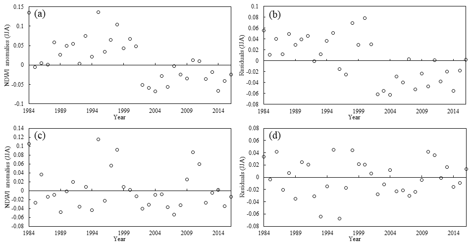
Figure 9The Beaverhead River (BVHR4) (a) NDWI anomalies over time and (b) NDWI anomaly–climate regression residuals over time. The Beaverhead River (BVHR2) (c) NDWI anomalies over time and (d) NDWI anomaly–climate regression residuals over time. The MK test for trends was significant (p<0.05) for (a) and (b) but not significant for (c) and (d). JJA: June, July and August.
3.3 Trends in river discharge
Growing-season riparian NDWI anomalies were significantly correlated (p<0.05) with growing-season river discharge at all seven USGS stream gages analyzed (Spearman correlation coefficient ranged between 0.55 along the Beaverhead River and Big Hole River and 0.82 along the Jefferson River; Table 7). In addition, all gages, except the Beaverhead River at the Twin Bridges gage, were significantly correlated with spring snowfall (Spearman p value < 0.05), the climate variable that showed the highest correlation on average between summer discharge and the climate variables considered in the analysis. Unlike the riparian reaches, we saw no temporal trend (1984–2016) in the growing-season river discharge for any of the seven gages evaluated. However, because the watershed is a snowmelt-driven system, we also tested if trends were restricted to the low-flow seasons (autumn and winter). During the autumn months (September, October and November) we observed a decline in river discharge at the Madison River (p<0.05) and Gallatin River (p<0.1) gages and an increase at the Big Hole River gage near Wisdom (p<0.05), which is near the upstream end of the Big Hole River (Table 7). During the winter months (December, January and February) we observed a decline in river discharge at the Madison river gage (p<0.05) and an increase in river discharge at the Beaverhead River near the Twin Bridges gage (p<0.1; Table 7).
Table 7River discharge characteristics for the US Geological Survey (USGS) gages used in the analysis. Summer (June, July and August) discharge was correlated with the summer normalized difference wetness index (NDWI) and spring snowfall (March–June) for the riparian reach adjacent to each gage, using the Spearman correlation. Temporal trends were quantified using the Mann–Kendall test for trends. Percentage discharge consumed and diverted is from the 2014 Water Plan (DNRC, 2014). JJA: June, July and August. SON: September, October and November. DJF: December, January and February. D: dam present at gage. D-US: dam upstream. ND: no dam or minimal flow regulation. N/A: data not available. SE: standard error. *: p<0.1. : p<0.05.

Across the western US, water withdrawals, diversions and impoundments associated with agriculture have contributed to riparian degradation (Goodwin et al., 1997; Klemas, 2014). In examining the multi-decadal trends in riparian wetness for a total of 158 km2 of riparian ecosystem across the UMH basin, we found long-term, significant drying along 8 of the 19 riparian reaches in this basin, including all three of the riparian reaches (the Jefferson, Madison and Gallatin rivers) at the confluence forming the Missouri River. In contrast, we did not observe trends in growing-season river discharge or climate variables over the same period. Shifts in land use, therefore, are a potential driver of the riparian condition across the UMH basin. Water withdrawals across the UMH basin are almost entirely surface water (99 %) and for irrigation (99 %; USGS, 1988; Dieter et al., 2018). We found only a moderate increase in total irrigated area over the period (+10.5 %). An increase in irrigated area is consistent with state-wide estimates over the same time period. The USDA Farm and Ranch Irrigation Survey (FRIS), for instance, documented an increase in the area of irrigated agriculture across Montana of 18.9 % between 1984 and 2013 (USDA, 1984, 2014). The persistence of drying trends in riparian vegetation after accounting for the influence of climate variability, and the correlation of riparian drying with basin-wide changes in irrigation practices, suggest that the complexities of agricultural water use and irrigation practices are likely to be contributing factors to the drying of riparian areas in this basin.
One source of uncertainty in our analysis is that at the Landsat scale (30 m) we were unable to confidently distinguish gravity-fed irrigation from non-center-pivot sprinkler irrigation, methods of irrigation that can be expected to show different rates of water efficiency. This source of uncertainty made it difficult to reach definitive conclusions about reach-scale changes in the consumptive water use using our data alone. However, our assumption of a transition away from gravity-fed irrigation and towards center-pivot irrigation is consistent with other comparable sources of data. Across Montana the FRIS surveys (1984 and 2013) documented an increase in the fraction irrigated with center pivot from 9 % to 30 %, a decrease in the fraction irrigated with gravity-fed irrigation from 77 % to 57 %, and a minimal change (<3 %) in the fraction of agriculture irrigated with non-center-pivot sprinklers (USDA, 1984, 2014). Across the UMH basin, the Montana Department of Revenue's FLU surveys documented a 17 % increase in center-pivot irrigation and a corresponding decrease in both sprinkler and gravity-fed irrigation between 2010 and 2017. Despite these ancillary datasets, however, it is possible that shifts from gravity-fed irrigation to non-center-pivot sprinkler irrigation have also contributed to changes in return flow and riparian condition. Using the irrigation data generated in this study, the shift in irrigation practices was concentrated along the Beaverhead, Jefferson and Gallatin rivers, all of which showed statistically significant drying in at least portions of their riparian reaches. Correspondingly, the Big Hole River sub-watershed, which is dominated by gravity-fed irrigated hay and pasture (Montana DNRC, 2014), showed the fewest hectares converted to center-pivot irrigation relative to other sub-watersheds over the study period, with no temporal trends in riparian wetness.
Shifts away from gravity-fed irrigation have been observed across the United States (Schaible, 2017). Advances in irrigation technology allow for water to be applied at the most appropriate timing in plant root zones to increase crop consumptive use of water and, therefore, crop yields (Falkenmark and Lannerstad, 2005; Ward and Pulido-Velazquez, 2008). However, despite the shift to more efficient irrigation methods, the total water applied to irrigated fields across the US remained largely stable over the same period (Schaible, 2017). This pattern may indicate that local water savings do not necessarily translate to the watershed scale. Increases in crop yields are linearly correlated with increases in evapotranspiration (Steduto et al., 2012) so that the reduction in water application is often offset by increases in evapotranspiration, specifically crop transpiration (Ward and Pulido-Velazquez, 2008; Grafton et al., 2018). A schematic of the potential impact of irrigation method on water cycling is shown in Fig. 10. Further, proposed water savings in per field water applications often fail to account for farm-level decisions and incentives (Ward and Pulido-Velazquez, 2008; Perry et al., 2017). Within the current water rights framework, more efficient water use can incentivize farmers to make changes to crop choices and crop rotation patterns or to increase the total area irrigated or the frequency of irrigation so that their water rights and usage are maintained and maximized (Pfeiffer and Lin, 2014; Grafton et al., 2018). If there is a local reduction in water usage downstream water users can more fully exercise their water rights so that there is no net reduction in water usage at the watershed scale (Ward and Pulido-Velazquez, 2008; Perry et al., 2017).
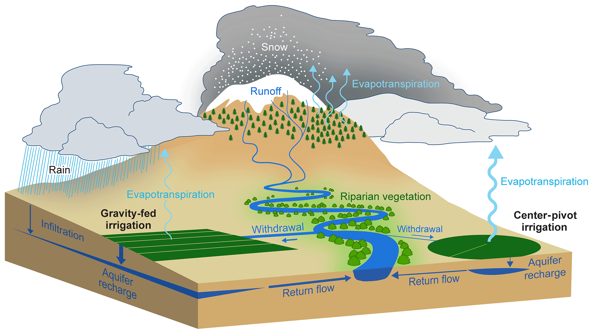
Figure 10A schematic showing the potential impacts of changing irrigation types. While shifting to center-pivot irrigation can be expected to reduce per field water applications, it can also be expected to increase evapotranspiration as well as decrease sub-surface return flow and aquifer recharge. Reduced withdrawal may not persist downstream but instead be used by the same farmer or a downstream user. Thicker and thinner lines are used to indicate more or less water, respectively.
Riparian and river condition for a given reach can be expected to be a function of its upstream river network, including water added and removed from upstream reaches, as well as upstream land uses (Ver Hoef and Peterson, 2012; Fritz et al., 2018). Biotic integrity, for example, has been shown to depend on upstream conditions (Schofield et al., 2018), which can extend tens of kilometers up the channel network (Van Sickle and Johnson, 2008). In consideration of this, the climate variables used to model temporal variability in riparian wetness were calculated as a function of each reach's total upstream contributing area. Similarly, we considered upstream accumulated changes in irrigation to help interpret trends in the NDWI anomaly–climate regression residuals. For instance, the total upstream increase in hectares of center-pivot irrigation over the period was found to be significantly different between reaches that showed a drying trend and those that did not. Landscape characteristics can also inform how a riparian ecosystem responds to changes in reach- or basin-scale hydrology. Well-drained soils and a higher Melton ruggedness number, characteristics significantly associated with the reach-scale riparian drying trends, can be expected to facilitate the return flow of excess irrigation water to the riparian corridor. These findings suggest that both reach-scale and upstream characteristics can influence how riparian vegetation will respond to changes in climate and land use.
While the presence of riparian drying trends in the NDWI anomaly–climate residuals indicated that the observed drying trends were not solely attributable to climate, climate variability was a significant predictor of the interannual variability in riparian wetness (e.g., Figs. 5 and 6), a finding documented in other geographic regions as well (e.g., Fu and Burgher, 2015; Nguyen et al., 2015; Huntington et al., 2016). Drought events, and the resilience of river and riparian ecosystems to these events, are a significant concern for stakeholders in the Upper Missouri Headwaters Basin (Montana DNRC, 2015; McEvoy et al., 2018). Evaluation of water rights and corresponding water withdrawals under drought conditions was beyond the scope of this study; however, our findings suggest that the conversion to center-pivot irrigation could amplify the impacts of reduced precipitation on riparian areas. Additionally, an increasing summer VPD could further increase crop water losses to evapotranspiration (Massmann et al., 2018), potentially exacerbating both the hydrological effect and salinization effect of irrigation conversion (Singh, 2015). We note, however, that climate and river discharge trends were quantified only to be compared with trends observed in riparian wetness over the same period (1984–2016). Because only partial climate and river discharge records were used, our findings regarding the presence or absence of trends in the climate and river discharge data should be interpreted with caution.
Despite only partial discharge records being utilized, one interesting finding was that over the same period a drying trend in riparian areas did not necessarily translate into a trend in river discharge. We can speculate that because the rivers are snowmelt dominated (Markstrom et al., 2016; Cross et al., 2017), during the summer months irrigation return flow may have an impact on riparian areas but could represent a relatively small percentage of summer flows. A comprehensive water budget or hydrological modeling approach, however, would be needed to quantify this and specifically to determine how anthropogenic activities may have a differential impact on riparian wetness relative to river discharge. Additionally, rivers across the basin vary in the amount of flow regulation from dams. For example, the Big Hole and Gallatin rivers are relatively unregulated, while the Madison River, Beaverhead River, Ruby River and Red Rock River are all regulated by large dams. The reservoirs above dams retain water during the spring runoff, reducing peak flows, and release more water in the autumn, changing a river's natural flow regime (Montana DNRC, 2014). It is possible that shifts in dam management and corresponding changes in flow regulation could contribute to trends in riparian wetness. However, river discharge (JJA) was significantly correlated with spring snowfall at eight of nine gages, suggesting that even with seasonal flow regulation, discharge along dammed rivers still typically represents interannual variability in climate.
Efforts to characterize the factors influencing variability and trends in riparian wetness are critical to maintain and restore riparian functionality. Healthy floodplains and riparian areas serve a number of functions, including slowing runoff, promoting local groundwater recharge and quickening the recovery of local groundwater storage post-drought (Montana DNRC, 2014). Spectral indices calculated from satellite imagery have been successfully used to monitor the response of riparian vegetation to variability in channel morphology (Henshaw et al., 2013; Hamdan and Myint, 2015) as well as changes induced by the installation of in-stream restoration structures (Hausner et al., 2018; Vanderhoof and Burt, 2018). While Landsat has been commonly used to examine multi-decadal trends in vegetation conditions (Goetz et al., 2005; McManus et al., 2012; White et al., 2017), because of the narrow, linear footprint of riparian ecosystems within human-influenced landscapes, efforts to apply Landsat time-series analysis to riparian systems have been limited (e.g., Henshaw et al., 2013; Hamden and Myint, 2015; Nguyen et al., 2015). Regional-scale Landsat efforts have tended to focus on changes to riparian extent rather than riparian trends in greenness or wetness (e.g., Jones et al., 2010; Macfarlane et al., 2017). Along river systems, however, the moderate resolution of Landsat can misrepresent riparian edges or fail to detect portions of the riparian corridor that are narrower than Landsat's minimum mapping unit, potentially influencing the calculated spectral patterns. In our analysis we minimized such errors by (1) restricting the analysis to rivers with riparian corridors large enough to be measured using Landsat and (2) using a consistent riparian area extent across the time series. It is clear, however, that sources of imagery with finer spatial resolution will be critical for riparian corridors too narrow to be monitored with Landsat imagery. To this end, data sources with increased spatial resolution are rapidly becoming more available and useful for monitoring water resources (e.g., Sentinel-2 or CubeSats; e.g., Vande Kamp et al., 2013; Gärtner et al., 2016; Cooley et al., 2017; Yang et al., 2017) but lack the multi-decadal data records provided by Landsat. This means that for larger riparian corridors, Landsat spectral indices remain a critical data source that can be used to characterize trends in riparian wetness as well as potentially quantify the impact of land use changes, including long-term shifts in irrigation methods, on riparian vegetation.
Riparian corridors provide valuable ecosystem functions including storing water; mitigating nutrients, pollutants and sediments; providing wildlife corridors; and influencing water temperature (Vivoni et al., 2006; Lees and Peres, 2008; Isaak et al., 2012). A drying trend in riparian areas across the Upper Missouri Headwaters Basin could lessen the effectiveness of these functions and shift the systems towards more drought-tolerant plant species that are less adapted to highly variable flow regimes (Capon et al., 2013; Catford et al., 2014). Although promoted as a more water-efficient approach, several recent studies have demonstrated a lack of catchment-scale water savings after farmers transitioned to center-pivot irrigation (Perry et al., 2017; Grafton et al., 2018). We were able to pair a Landsat time-series analysis with climate and agricultural data to document a statistically significant drying trend, not explained by climate variability, along nearly half (42 %) of riparian reaches in the Upper Missouri Headwaters Basin. The riparian reaches experiencing drying trends tended to have more upstream agriculture and greater shifts toward center-pivot irrigation, but the correlations between agricultural activities and riparian wetness were imperfect, suggesting that the upstream river network, as well as other reach-scale characteristics such as the riparian species or the geology or soil characteristics, also influence the response of a riparian reach to changes in water withdrawal. In addition, the drying trends in riparian ecosystems were not observed in the snowmelt-driven river discharge (JJA), a finding that should be explored further using hydrological models. Maintaining and improving riparian functionality across watersheds dominated by agricultural activity will require not only more efforts to track temporal trends in riparian vegetation but also more efforts to separate out the relative influence of climate and anthropogenic activities.
Following publication, the data related to this publication will be published in the US Geological Survey's ScienceBase catalog (https://doi.org/10.5066/P976LZ2G; Vanderhoof et al., 2019).
MKV, JRC and LCA designed the study; MKV and JRC derived the input datasets; MKV performed the analysis; and MKV, JRC and LCA wrote the paper.
The authors declare that they have no conflict of interest.
We thank Haley Distler for her assistance in delineating the riparian corridor and Jeremey Havens for his assistance in generating the hydrology schematic. We also thank Ken Fritz, Robert Payn, Richard Marinos and the anonymous reviewer for their insightful comments on earlier versions of this paper. Any use of trade, firm or product names is for descriptive purposes only and does not imply endorsement by the US government. This publication represents the views of the authors and does not necessarily reflect the views or policies of the US EPA.
This project was funded by the US Geological Survey Land Resources and Land Change Science Program as well as by a US EPA Region 8 RARE grant, entitled “Building drought resiliency and watershed prioritization using natural water storage techniques”, through the associated interagency agreement (DW-014-92475401-0).
This paper was edited by Nandita Basu and reviewed by Richard Marinos and one anonymous referee.
Ascione, A., Cinque, A., Miccadei, E., Villani, F., and Berti, C.: The Plio-Quaternary uplift of the Apennine chain: New data from the analysis of topography and river valleys in Central Italy, Geomorphology, 102, 105–118, 2008.
Bauder, J. W.: Early season alfalfa irrigation strategies, Montana State University Extension, Bozeman, MT, available at: http://waterquality.montana.edu/farm-ranch/irrigation/alfalfa/early.html, last access: 19 November 2018.
Boutin, C. and Belanger, J. B.: Importance of riparian habitats to flora conservation in farming landscapes of southern Quebec, Canada, Agr. Ecosyst. Environ., 94, 73–87, 2003.
Capon, S. J., Chambers, L. E., Mac Nally, R., Naiman, R. J., Davies, P., Marshall, N., Pittock, J., Reid, M., Capon, T., Douglas, M., Catford, J., Baldwin, D. S., Stewardson, M., Roberts, J., Parsons, M., and Williams, S. E.: Riparian ecosystems in the 21st century: Hotspots for climate change adaptation?, Ecosystems, 16, 359–381, 2013.
Carrillo-Guerrero, Y., Glenn, E. P., and Hinojosa-Huerta, O.: Water budget for agricultural and aquatic ecosystems in the delta of the Colorado River, Mexico: Implications for obtaining water for the environment, Ecol. Eng., 59, 41–51, 2013.
Catford, J. A., Morris, W. K., Vesk, P. A., Gippel, C. J., and Downes, B. J.: Species and environmental characteristics point to flow regulation and drought as drivers of riparian plant invasion, Biodiv. Res., 20, 1084–1096, 2014.
Chatterjee, C., Kumar, R., Chakravorty, B., Lohani, A. K., and Kumar, S.: Integrating remote sensing and GIS techniques with groundwater flow modeling for assessment of waterlogged areas, Water Resour. Manage., 19, 539–554, 2005.
Chowdary, V. M., Vinu Chandran, R., Neeti, N., Bothale, R. V., Srivastava, Y. K., Ingle, P., Ramakrishnan, D., Dutta, D., Jeyaram, A., Sharma, J. R., and Singh, R.: Assessment of surface and sub-surface waterlogged areas in irrigation command areas of Bihar state using remote sensing and GIS, Agr. Water Manage., 95, 754–766, 2008.
Clancy, C. G.: Effects of dewatering on spawning by Yellowstone cutthroat trout in tributaries of the Yellowstone River, Montana, Am. Fish. Soc. Symp., 4, 37–41, 1988.
Clifford, M.: Preserving stream flows in Montana through the Constitutional Public Trust Doctrine: An underrated solution, Publ. Land Law Rev., 16, 117–135, 1995.
Cohen, J.: Statistical Power Analysis for the Behavioral Sciences, 2nd Edn., Lawrence Erlbaum Associates, New York City, 1988.
Cooley, S., Smith, L., Stepan, L., and Mascaro, J.: Tracking dynamic northern surface water changes with high-frequency Planet CubeSat imagery, Remote Sens., 9, 1306, https://doi.org/10.3390/rs9121306, 2017.
Crétaux, J.-F., Biancamaria, S., Arsen, A., Bergé-Nguyen, M., and Becker, M.: Global surveys of reservoirs and lakes from satellites and regional application to the Syrdarya river basin, Environ. Res. Lett., 10, 015002, https://doi.org/10.1088/1748-9326/10/1/015002, 2015.
Cross, W. F., LaFave, J., Leone, A., Lonsdale, W., Royem, A., Patton, T., and McGinnis, S.: Chapter 3, Water and climate change in Montana, in: the 2017 Montana Climate Assessment, edited by: Whitlock, C., Cross, W. F., Maxwell, B., Silverman, N. and Wade, A. A., Helena, MT, 77 pp., 2017.
Cunningham, S. C., Thomson, J. R., Mac Nally, R., Read, J., and Baker, P. J.: Groundwater change forecasts widespread forest dieback across an extensive floodplain system, Freshwater Biol., 56, 1494–1508, 2011.
Dieter, C. A., Linsey, K. S., Caldwell, R. R., Harris, M. A., Ivahnenko, T. I., Lovelace, J. K., Maupin, M. A., and Barber, N. L. Estimated use of water in the United States county-level data for 2015, US Geological Survey, Reston, VA, 2018.
Dragoni, W. and Sukhiga, B. S.: Climate change and groundwater: a short review, Geol. Soc. Lond. Spec. Publ., 288, 1–12, https://doi.org/10.1144/SP288.1, 2008.
Duffield, J., Neher, C. J., and Brown, T. C.: Recreation benefits of instream flow: Application to Montana Big Hole and Bitterroot Rivers, Water Resour. Res., 28, 2169–2181, 1992.
Falkenmark, M. and Lannerstad, M.: Consumptive water use to feed humanity – curing a blind spot, Hydrol. Earth Syst. Sci., 9, 15–28, https://doi.org/10.5194/hess-9-15-2005, 2005.
Fritz, K. M., Schofield, K. A., Alexander, L. C., McManus, M. G., Golden, H. E., Lane, C. R., Kepner, W. G., LeDuc, S. D., DeMeester, J. E., and Pollard, A. I.: Physical and chemical connectivity of streams and riparian wetlands to downstream waters: a synthesis, J. Am. Water Resour. Assoc., 54, 323–345, 2018.
Fu, B. and Burgher, I.: Riparian vegetation NDVI dynamics and its relationship with climate, surface water and groundwater, J. Arid Environ., 113, 59–68, 2015.
Gao, B.: NDWI – a normalized difference water index for remote sensing of vegetation liquid water from space, Remote Sens. Environ., 58, 257–266, 1996.
Gärtner, P., Förster, M., and Kleinschmit, B.: The benefit of synthetically generated RapidEye and Landsat 8 data fusion time series for riparian forest disturbance monitoring, Remote Sens. Environ., 177, 237–247, 2016.
Gesch, D., Oimoen, M., Greenlee, S., Nelson, C., Steuck, M., and Tyler, D.: The National Elevation Dataset, Photogramm. Eng. Remote Sens., 68, 5–11, 2002.
Gilbert, R. O.: Statistical Methods for Environmental Pollution Monitoring, Wiley, NY, 1987.
Goetz, S. J., Bunn, A. G., Fiske, G. J., and Houghton, R. A.: Satellite-observed photosynthetic trends across boreal North America associated with climate and fire disturbance, P. Natl. Acad. Sci. USA, 102, 13521–13525, 2005.
Goklany, I. M.: Comparing 20th century trends in U.S. and global agricultural water and land use, Water Int., 27, 321–329, 2002.
Goodwin, C. N., Hawkins, C. P., and Kershner J. L.: Riparian restoration in the western United States: overview and perspective, Restor. Ecol., 5, 4–14, 1997.
Gosnell, H., Haggerty, J. H., and Byorth, P. A.: Ranch ownership change and new approaches to water resource management in southwestern Montana: implications for fisheries, J. Am. Water Resour. Assoc., 43, 990–1003, 2007.
Goudie, A. S.: Global warming and fluvial geomorphology, Geomorphology, 79, 384–394, 2006.
Grafton, R. Q., Williams, J., Perry, C. J., Molle, F., Ringler, C., Steduto, P., Udall, B., Wheeler, S. A., Wang, Y., Garrick, D., and Allen, R. G.: The paradox of irrigation efficiency, Science, 361, 748–750, 2018.
Gude, P. H., Hansen, A. J., Rasker, R., and Maxwell, B.: Rates and drivers of rural residential development in the Greater Yellowstone, Landsc. Urban Plan., 77, 131–151, 2006.
Hackett, O. M., Visher, F. N., McMurtrey, R. G., and Steinhilber, W. L.: Geology and ground water resources of the Gallatin Valley, Gallatin County, Montana, US Geological Survey Water-Supply Paper 1482, United States Government Printing Office, Washington, D.C., 282 pp., 1960.
Hamdan, A. and Myint, S. W.: Biogeomorphic relationships and riparian vegetation changes along altered ephemeral stream channels: Florence to Marana, Arizona, Prof. Geogr., 68, 26–38, 2015.
Hamed, K. H. and Rao, A. R.: A modified Mann–Kendall trend test for autocorrelated data, J. Hydrol., 204, 182–196, 1998.
Hansen, A. J., Rasker, R., Maxwell, B., Rotella, J. J., Johnson, J. D., Parmenter, A. W., Langner, U., Cohen, W. B., Lawrence, R. L., and Kraska, P. V.: Ecological causes and consequences of demographic change in the new west, Bioscience, 52, 151–162, 2002.
Hastie, T., Tibshirani, R., and Friedman, J.: The Elements of Statistical Learning, Springer, New York, 2009.
Hausner, M. B., Huntington, J. L., Nash, C., Morton, C., McEvoy, D. J., Pilliod, D. S., Hegewisch, K. C., Daudert, B., Abatzoglou, J. T., and Grant, G.: Assessing the effectiveness of riparian restoration projects using Landsat and precipitation data from the cloud-computing application http://climateengine.org/, Ecolog. Eng., 120, 432–440, 2018.
Henshaw, A. J., Gurnell, A. M., Bertoldi, W., and Drake, N. A.: An assessment of the degree to which Landsat TM data can support the assessment of fluvial dynamics, as revealed by changes in vegetation extent and channel position, along a large river, Geomorphology, 202, 74–85, 2013.
Homer, C., Dewitx, J., Yang, L., Jin, S., Danielson, P., Xian, G., Coulston, J., Herold, N., Wickham, J., and Megown, K.: Completion of the 2011 National Land Cover Database for the conterminous United States – Representing a decade of land cover change information, Photogram. Eng. Remote Sens., 81, 345–354, 2015.
Hughes, F. M. R., Colston, A., and Mountford, J. O.: Restoring riparian ecosystems: The challenge of accommodating variability and designing restoration trajectories, Ecol. Soc., 10, 1–22, 2005.
Huntington, J., McGwire, K., Morton, C., Snyder, K., Peterson, S., Erckson, T., Niswonger, R., Carroll, R., Smith, G., and Allen, R.: Assessing the role of climate and resource management on groundwater dependent ecosystem changes in arid environments with the Landsat archive, Remote Sens. Environ., 185, 186–197, 2016.
Hurvich, C. M. and Tsai, C. L.: Regression and time series model selection in small samples, Biometrika, 76, 297–307, 1989.
Isaak, D. J., Wollrab, S., Horan, D., and Chandler, G.: Climate change effects on stream and river temperatures across the northwest U.S. from 1980–2009 and implications for salmonid fishes, Climatic Change, 113, 499–524, 2012.
Jones, K. B., Edmonds, C. E., Slonecker, E. T., Wickham, J. D., Neale, A. C., Wade, T. G., Riiters, K. H., and Kepner, W. G.: Detecting changes in riparian habitat conditions based on patterns of greenness change: A case study from the Upper San Pedro River Basin, USA, Ecol. Indic., 8, 89–99, 2008.
Jones, K. B., Slonecker, E. T., Nash, M. S., Neale, A. C., Wade, T. G., and Hamann, S.: Riparian habitat changes across the continental United States (1972–2003) and potential implications for sustaining ecosystem services, Landsc. Ecol., 25, 1261–1275, 2010.
Kendall, M. G.: Rank Correlation Methods, Griffin, London, 1975.
Kendy, E. and Bredehoeft, J. D.: Transient effects of groundwater pumping and surface-water irrigation returns on streamflow, Water Resour. Res., 42, W08415, https://doi.org/10.1029/2005WR004792, 2006.
Kerkvliet, J., Nowell, C., and Lowe, S.: The economic value of the Greater Yellowstone's Blue-Ribbon fishery, N. Am. J. Fish. Manage., 22, 418–424, 2002.
Klemas, V.: Remote sensing of riparian and wetland buffers: an overview, J. Coast. Res., 30, 869–880, 2014.
Lees, A. C. and Peres, C. A.: Conservation value of remnant riparian forests corridors of varying quality for amazonian birds and mammals, Conserv. Biol., 2, 439–449, 2008.
Leyk, S. and Uhl, J. H.: Historical built-up intensity layer series for the U.S. 1810–2015, Harvard Dataverse, V1, https://doi.org/10.7910/DVN/1WB9E4, 2018.
Liaw, A. and Wiener, M.: Breiman and Cutler's random forests for classification and regression, R package version 4.6-12, R Foundation for Statistical Computing, Vienna, Austria, 1–29, 2015.
Lowrance, R., Todd, R., Fail Jr., J., Hendrickson Jr., O., Leonard, R., and Asmussen, L.: Riparian forests as nutrient filters in agricultural watersheds, Bioscience, 34, 374–377, 1984.
Macfarlane, W. W., Gilbert, J. T., Jensen, M. L., Gilbert, J. D., Hough-Snee, N., McHugh, P. A., Wheaton, J. M., and Bennett, S. N.: Riparian vegetation as an indicator of riparian condition: detecting departures from historic condition across the North American West, J. Environ. Manage., 202, 447–460, 2017.
Mann, H. B.: Nonparametric tests against trend, Econometrica, 13, 245–259, 1945.
Markstrom, S. L., Hay, L. E., and Clark, M. P.: Towards simplification of hydrologic modeling: identification of dominant processes, Hydrol. Earth Syst. Sci., 20, 4655–4671, https://doi.org/10.5194/hess-20-4655-2016, 2016.
Massmann, A., Gentine, P., and Lin, C.: When does vapor pressure deficit drive or reduce evapotranspiration?, Hydrol. Earth Syst. Sci. Discuss., https://doi.org/10.5194/hess-2018-553, in review, 2018.
McEvoy, J., Bathke, D. J., Burkardt, N., Cravens, A. E., Haigh, T., Hall, K. R., Hayes, M. J., Jedd, T., Podebradska, M., and Wickham, E.: Ecological drought: Accounting for the non-human impacts of water shortage in the Upper Missouri Headwaters Basin, Montana, USA, Resources, 7, 1–17, 2018.
McFeeters, S. K.: The use of normalized difference water index (NDWI) in the delineation of open water features, Internat, J. Remote Sens., 17, 1425–1432, 1996.
McFeeters, S. K.: Using the Normalized Difference Water Index within a geographic information system to detect swimming pools for mosquito abatement: a practical approach, Remote Sens., 5, 3544–3561, 2013.
McManus, K. M., Morton, D. C., Masek, J. G., Wang, D., Sexton, J. O., Nagol, J. R., Ropars, P., and Boudreau, S.: Satellite-based evidence for shrub and graminoid tundra expansion in northern Quebec from 1986 to 2010, Global Change Biol., 18, 2313–2323, 2012.
Melton, M. A.: The geomorphic and paleoclimatic significance of alluvial deposits in southern Arizona, J. Geol., 73, 1–38, 1965.
Montana DNRC – Montana Department of Natural Resources and Conservation: Upper Missouri Basin Water Plan 2014, Montana Department of Natural Resources and Conservation, Helena, MT, 219 pp., 2014.
Montana DNRC – Montana Department of Natural Resources and Conservation: Montana State Water Plan, Montana Department of Natural Resources and Conservation, Helena, MT, 64 pp., 2015.
Montana Drought Demonstration Partners: A Workplan for Drought Resilience in the Missouri Headwaters Basin: A National Demonstration Project, available at: http://dnrc.mt.gov/divisions/water/management/docs/surface-waterstudies/workplan_drought_resilience~missouri_headwaters.pdf (last access: 1 August 2019), 2015.
Murphy, M. A., Evans, J. S., and Storfer, A.: Quantifying Bufo boreas connectivity in Yellowstone National Park with landscape genetics, Ecology, 91, 252–261, 2010.
Naiman, R. J., Décamps, H., and McClain, M. E. Riparia: ecology, conservation and management of streamside communities, Academic Press, New York, 2005.
Nguyen, U., Glen, E. P., Nagler, P. L., and Scott, R. L.: Long-term decrease in satellite vegetation indices in response to environmental variables in an iconic desert riparian ecosystem: The Upper San Pedro, Arizona, United States, Ecohydrology, 8, 610–625, 2015.
Nilsson, C. and Berggren, K.: Alterations of riparian ecosystems caused by river regulation, Bioscience, 50, 783–792, 2000.
NOAA NCDC – National Climatic Data Center: Data Tools: 1981–2010 Normals, available at: http://www.ncdc.noaa.gov/cdo-web/datatools/normals (last access: 3 October 2018), 2014.
NSIDC – National Snow and Ice Data Center: All about snow, National Snow and Ice Data Center, Boulder, CO, 2018.
Pederson, G. T., Gray, S. T., Woodhouse, C. A., Betancourt, J. L., Fagre, D. B., Littell, J. S., Watson, E., Luckman, B. H., and Graumlich, L. J.: The unusual nature of recent snowpack declines in the North American Cordillera, Science, 333, 332–335, 2011.
Pederson, G. T., Betancourt, J. L., and McCabe, G. J.: Regional patterns and proximal causes of the 60 recent snowpack decline in the Rocky Mountains, U.S., Geophys. Res. Lett., 40, 1811–1816, 2013.
Perry, C., Steduto, P., and Karejeh, F.: Does improved irrigation technology save water? A review of the evidence, Food and Agriculture Organization of the United Nations, Cairo, Egypt, 57 pp., 2017.
Peterson, E. E.: STARS: Spatial Tools for the Analysis of River Systems version 2.0.6 – a tutorial, Queensland University of Technology, Brisbane, Australia, 47 pp., 2017.
Peterson, J. M. and Ding, Y.: Economic adjustments to groundwater depletion in the high plains: Do water-saving irrigation systems save water?, Am. J. Agric. Econ., 87, 147–159, 2005.
Pfeiffer, L. and Lin, C. Y. C.: Does efficient irrigation technology lead to reduced groundwater extraction? Empirical evidence, J. Environ. Econ. Manage., 67, 189–208, 2014.
Poff, N. L., Allan, J. D., Bain, M. B., Karr, J. R., and Prestagaard, K. L.: The natural flow regime, BioScience, 47, 769–784, 1997.
Poole, G. C. and Berman, C. H.: An ecological perspective on in-stream temperature: Natural heat dynamics and mechanisms of human-caused thermal degradation, Environ. Manage., 27, 787–802, 2001.
PRISM Climate Group, Oregon State University: PRISM Climate Data, available at: http://prism.oregonstate.edu, last access: 27 June 2018.
Richardson, D. M., Holmes, P. M., Esler, K. J., Galatowitsch, S. M., Stromberg, J. C., Kirkman, S. P., Pysek, P., and Hobbs, R. J.: Riparian vegetation: Degradation, alien plant invasions, and restoration prospects, Divers. Distrib., 13, 126–139, 2007.
Rood, S. B., Pan, J., Gill, K. M., Franks, C. G., Samuelson, G. M., and Shepherd, A.: Declining summer flows of Rocky Mountain rivers: changing seasonal hydrology and probable impacts on floodplain forests, J. Hydrol., 349, 397–410, 2008.
Schaible, G.: Understanding irrigated agriculture, Statistic: Farm Practices & Management, US Department of Agriculture, Economic Research Service, Washington, D.C., USA, 6 pp., 2017.
Schaible, G. D. and Aillery, M. P.: Water conservation in irrigated agriculture: Trends and challenges in the face of emerging demands, EIB-99, US Department of Agriculture, Economic Research Service, Washington, D.C., USA, 2012.
Schofield, K. A., Alexander, L. C., Ridley, C. E., Vanderhoof, M. K., Fritz, K. M., Autrey, B., DeMeester, J., Kepner, W. G., Lane, C. R., Leibowitz, S., and Pollard, A. I.: Biota connect aquatic habitats throughout freshwater ecosystem mosaics, J. Am. Water Resour. Assoc., 54, 372–399, https://doi.org/10.1111/1752-1688.12634, 2018.
Shafroth, P. B., Stromberg, J. C., and Patten, D. T.: Riparian vegetation response to altered disturbance and stress regimes, Ecol. Appl., 12, 107–123, 2002.
Singh, A.: Soil salinization and waterlogging: A threat to environment and agricultural sustainability, Ecol. Indic., 57, 128–130, 2015.
Slagle, S. E.: Geohydrologic conditions and land use in the Gallatin Valley, southwestern Montana, 1992–93, US Geological Survey Water-Resources Investigations Report 95-4034, US Geological Survey, Washington, D.C., USA, p. 2, 1995.
Soil Survey Staff, Natural Resources Conservation Service, United States Department of Agriculture, Soil Survey Geographic (SSURGO): Database for Montana, available at: https://sdmdataaccess.sc.egov.usda.gov, last access: 25 June 2018.
Steduto, P., Hsiao, T. C., Fereres, E., and Raes, D.: Crop yield response to water, Irrigation and Drainage Paper 66, Food and Agricultural Organization, Rome, Italy, 505 pp., 2012.
Stromberg, J. C.: Restoration of riparian vegetation in the south-western United States: Importance of flow regimes and fluvial dynamism, J. Arid Environ., 49, 17–34, 2001.
Stromberg, J. C., Lite, S. J., Rychener, T. J., Levick, L. R., Dixon, M. D., and Watts, J. M.: Status of the riparian ecosystem in the Upper San Pedro River, Arizona: Application of an assessment model, Environ. Monit. Assess., 115, 145–173, 2006.
Sweeney, B. W., Bott, T. L., Jackson, J. K., Kaplan, L. A., Newbold, J. D., Standley, L. J, Horwitz, R. J., and Hession, W. C.: Riparian deforestation, stream narrowing, and loss of stream ecosystem services, P. Natl. Acad. Sci. USA, 101, 14132–14137, 2004.
Theobald, D. M., Norman, J. B., Peterson, E., Ferraz, S., Wade, A., and Sherburne, M. R.: Functional linkage of water basins and streams (FLoWS) v1 user's guide: ArcGIS tools for network-based analysis of freshwater ecosystems, Natural Resource Ecology Lab, Colorado State University, Fort Collins, CO, 43 pp., 2006.
Tucker, C. J.: Red and photographic infrared linear combinations for monitoring vegetation, Remote Sens. Environ., 8, 127–150, 1979.
USBR – US Bureau of Reclamation: Climate Change Analysis for the Missouri River Basin, Technical Memorandum No. 86-68210-2012-03, US Bureau of Reclamation, Washington, D.C., USA, 2012.
USDA – US Department of Agriculture: 1984 Farm and Ranch Irrigation Survey (2013), AG84-SR-1, US Department of Commerce, Bureau of the Census, Washington, D.C., USA, 1984.
USDA – US Department of Agriculture: Farm and Ranch Irrigation Survey (2013), Volume 3, Special Studies, Part 1, AC-12-SS-1, Washington, D.C., USA, 2014.
USDA – US Department of Agriculture: National Agricultural Statistics Service Cropland Data Layer, USDA-NASS, Washington, D.C., available at: https://nassgeodata.gmu.edu/CropScape/, last access: 5 November 2018.
USGS – US Geological Society: U.S. Geological Survey, Water Resources of the United States, ScienceBase Data Publication, Reston, VA, available at: https://www.sciencebase.gov/catalog/item/57361cc8e4b0dae0d5df6d22 (last access: 22 November 2018), 1988.
Vanderhoof, M. K. and Burt, C.: Applying high-resolution imagery to evaluate restoration-induced changes in stream condition, Missouri River Headwaters Basin, Montana, Remote Sens., 10, 913, https://doi.org/10.3390/rs10060913, 2018.
Vanderhoof, M. K. and Lane, C. R.: The potential role of very high-resolution imagery to characterize lake, wetland and stream systems across the Prairie Pothole Region, United States, Int. J. Remote Sens., https://doi.org/10.1080/01431161.2019.1582112, in press, 2019.
Vanderhoof, M. K., Christensen, J. C., and Alexander, L. C.: Data release for the influence of multi-decadal land use, irrigation practices and climate on riparian corridors across the Upper Missouri River headwaters basin, Montana, US Geological Survey data release, https://doi.org/10.5066/P976LZ2G, 2019.
Vande Kamp, K., Rigge, M., Troelstrup Jr., N. H., Smart, A. J., and Wylie, B.: Detecting channel riparian vegetation response to best-management-practices implementation in ephemeral streams with the use of Spot high-resolution visible imagery, Range. Ecol. Manage., 66, 63–70, 2013.
Van Sickle, J. and Johnson, C. B.: Parametric distance weighting of landscape influence on streams, Landsc. Ecol., 23, 427–438, 2008.
Ver Hoef, J. M. and Peterson, E. E.: A moving average approach for spatial statistical models of stream networks, J. Am. Stat. Assoc., 105, 6–18, 2012.
Vivoni, E., Bowman, R. S., Wychkoff, R. L., Jakubowski, R. T., and Richards, K. E.: Analysis of a monsoon flood event in an ephemeral tributary and its downstream hydrologic effects, Water Resour. Res., 42, W03404, https://doi.org/10.1029/2005WR004036, 2006.
Ward, F. A. and Pulido-Velazquez, M.: Water conservation in irrigation can increase water use, P. Natl. Acad. Sci. USA, 105, 18215–18220, 2008.
White, J. C., Wulder, M. A., Hermosilla, T., Coops, N. C., and Hobart, G. W.: Nationwide annual characterization of 25 years of forest disturbance and recovery for Canada using Landsat time series, Remote Sens. Environ., 194, 303–321, 2017.
Wisser, D., Frolking, S., Douglas, E. M., Fekete, B. M., Vörösmarty, C. J., and Schumann, A. H.: Global irrigation water demand: variability and uncertainties arising from agricultural and climate data sets, Geophys. Res. Lett., 35, 1–5, 2008.
Yang, X., Zhao, S., Qin, X., Zhao, N., and Liang, L.: Mapping of urban surface water bodies from Sentinel-2 MSI imagery at 10 m resolution via NDWI-based image sharpening, Remote Sens., 9, 596, 2017.