2.1 Reservoir index (RI)

Intuitively, the larger the reservoir capacity relative to the flow of a downstream gauging station, the greater the possible effects of the reservoir on the streamflow regime. To quantify reservoir-induced alterations to the downstream streamflow regime, Batalla et al. (2004) proposed an impounded runoff index (IRI), which is a ratio of reservoir capacity (RC) to (unimpaired) mean annual runoff ($\stackrel{\mathrm{‾}}{Q}$) at the gauge station, denoted as $\mathrm{IRI}=\mathrm{RC}/\stackrel{\mathrm{‾}}{Q}$. For a single reservoir, the IRI is a good indicator of the extent to which a reservoir alters streamflow. To analyze the effects of a multi-reservoir system on the downstream flood frequency, López and Francés (2013) proposed a dimensionless reservoir index. In this study, we additionally considered the effects of reservoir sediment deposition on the reservoir capacity. In accordance with López and Francés (2013), the RI for a downstream gauging station is defined as

where N is the total number of reservoirs upstream of the gauge station, A_i is the total basin area upstream of the ith reservoir, A_T is the total basin area upstream of the gauge station, RC_i is the total storage capacity of the ith reservoir, and LR_i is the loss rate (%) of RC_i due to the sediment deposition (Supplement). Equation (1) indicates that for a reservoir system consisting of small- and middle-sized reservoirs, the RI for the downstream gauging station is generally less than 1. However, for a system with some large reservoirs, such as multi-year regulating storage reservoirs, the RI of the downstream gauging station near this system may be close to 1 or higher.

2.2 Rainfall–reservoir composite index (RRCI)

In addition to the reservoir capacity, the MARI, which is an event of continuous multiday multivariate rainfall that forms the inflow event that will be regulated by the reservoir system to become the downstream extreme flow, is a key constraint for scheduling the reservoir system. In this study, to add the antecedent rainfall effects into the new indicator of reservoir effects, five variables were used to describe the MARI: the maximum M (the maximum daily rainfall in the MARI), the intensity I (the mean daily rainfall in the MARI), the volume V (the total daily rainfall in the MARI), the timing T (the end time of MARI during that year), and the distance L (the distance between the rainfall center and the outlet). The reason that M, I, V, and L were selected is because these variables will determine the peak, the total volume, and the peak appearance time of an inflow event. The variable T is utilized to capture information regarding the remaining storage capacity due to staged operation strategies during flood season used in some reservoirs. For the operation strategy that consists of increasing the flood limit water level in stages, it is expected that if the timing of the MARI is near the end of the flood season, the downstream AMDF will be less affected by reservoirs. This is because of the lesser remaining capacity during this period. The MARI variables that are selected to construct the new indicator are hereafter referred to as the scheduling-related MARI variables (denoted as $X_{\mathrm{1}},X_{\mathrm{2}},\mathrm{\dots },X_d$). The extraction procedure of the MARI is detailed in Sect. 3.2.

A new index is proposed in this study, the RRCI, to more comprehensively assess the effects of reservoirs on floods by incorporating the effects of the MARI. This index is defined as

where $P_{\mathrm{MARI}}^{\vee }$ is the OR joint exceedance probability (OR-JEP), which is the probability that any one of the given set of values ($x_{\mathrm{1}},x_{\mathrm{2}},\mathrm{\dots },x_d$) for the scheduling-related MARI variables will be exceeded. Here, the OR-JEP acts as a rainfall index for measuring the MARI effects. The lower this probability, the greater effects the MARI has on reservoir operation. Then, it is expected that downstream floods could possibly obtain relatively large values and vice versa. Figure 2 illustrates the relationship in Eq. (2), which shows that the RRCI is conditional on both the OR-JEP and the RI. Equation (2) can then be expressed as

where F(⋅) is the cumulative distribution function (CDF) that determines the dependence relationship of the variables. The expectation of the RRCI is as follows:

In addition, for the OR case, the following is true:

Equations (3) and (5) indicate that, in addition to the RI, the RRCI is related to the number and the dependence relationship of the scheduling-related MARI variables. To obtain a reasonable RRCI, the unrelated MARI variables should not be incorporated. In this study, the number of MARI variables that were incorporated was no more than four to avoid a “dimension disaster” in modeling their dependence. To select the scheduling-related MARI variables, a three-step selection procedure was used that included the following: (1) selecting four variables from the five MARI variables by testing the significance of the Pearson correlation between the MARI variables and the AMDF, (2) calculating the RRCI for all possible subsets of the four variables using the d-dimensional ($d=\mathrm{1},\mathrm{2},\mathrm{3},\mathrm{4})$ copulas, then finally (3) identifying the variables by using the highest rank correlation coefficient between the RRCI and the AMDF. The construction method of the d-dimensional ($d=\mathrm{2},\mathrm{3},\mathrm{4}$) distribution $F\left(x_{\mathrm{1}},x_{\mathrm{2}},\mathrm{\dots },x_d\right)$ is described in the following subsection.

Figure 2Relationship in Eq. (2). (a) The contour plot of the RRCI against both the RI and the OR-JEP; panel (b) is the function curves of the RRCI against the OR-JEP under different values of RI.

Download

2.3 C-vine Copula model

In this subsection, a C-vine Copula model for the construction of the continuous d-dimensional distribution $F\left(x_{\mathrm{1}},x_{\mathrm{2}},\mathrm{\dots },x_d\right)$ is clarified. Sklar's theorem (Sklar, 1959) showed that for a continuous d-dimensional distribution, the one-dimensional marginals and dependence structure can be separated, and the dependence can be represented using a copula formula as follows:

where u_i is the univariate marginal distribution of X_i, C(⋅) is the copula function, θ_c is the copula parameter vector, θ_i is the parameter vector of the ith marginal distribution, and $\mathit{\theta }=\left({\mathit{\theta }}_{\mathrm{c}},{\mathit{\theta }}_{\mathrm{1}},{\mathit{\theta }}_{\mathrm{2}},\mathrm{\dots },{\mathit{\theta }}_d\right)$ is the parameter vector of the entire d-dimensional distribution. Thus, the construction of $F\left(x_{\mathrm{1}},x_{\mathrm{2}},\mathrm{\dots }{x}_d\right)$ can be separated into two steps: the first is the modeling of the univariate marginals, and the second is the modeling of the dependence structure. For the first step, the empirical distribution is used as the univariate marginal distributions, and the change points of the variables are tested using the Pettitt test (Pettitt, 1979). Then, if there are any, the marginal distribution and the change point will be addressed using the estimation method (Xiong et al., 2015). Then, for the second step, the copula construction for the dependence modeling is based on the pair-copula construction method, which has been widely used in previous research (Aas et al., 2009; Xiong et al., 2015). According to Aas et al. (2009), the joint density function $f\left(x_{\mathrm{1}},x_{\mathrm{2}},\mathrm{\dots },x_d\right)$ is written as

The d-dimensional copula density $c_{\mathrm{1}\mathrm{\dots }d}\left(u_{\mathrm{1}},u_{\mathrm{2}},\mathrm{\dots },u_d\right)$, which can be decomposed into $d(d-\mathrm{1})/\mathrm{2}$ bivariate copulas, corresponding to a C-vine structure, is given by

where $c_{j,i+j\left|\mathrm{1},\mathrm{\dots },j-\mathrm{1}\right.}$ is the density function of a bivariate pair copula, and ${\mathit{\theta }}_{j,i\left|\mathrm{1},\mathrm{\dots },j-\mathrm{1}\right.}$ is a parameter vector of the corresponding bivariate pair copula. Therefore, the marginal conditional distribution is

where $C_{i+j,j-\mathrm{1}\left|\mathrm{1},\mathrm{\dots },j-\mathrm{2}\right.}$ is a bivariate copula distribution function. The maximum dimensionality covered in this study was four. Thus for a four-dimensional copula (of which the decomposition is shown in Fig. 3), the general expression of Eq. (8) is

Figure 3Decomposition of a C-vine copula using four variables and three trees (denoted by T1, T2, and T3).

Download

2.4 Covariate-based nonstationary frequency analysis using the Bayesian estimation

The covariate-based extreme frequency analysis has been widely used (Villarini et al., 2009; Ouarda and El-Adlouni, 2011; López and Francés, 2013; Xiong et al., 2018). According to these studies, five distributions, namely the gamma (GA), Weibull (WEI), lognormal (LOGNO), Gumbel (GU), and the generalized extreme value (GEV) distribution, were used as candidate distributions in this study. In addition, their density functions, the corresponding moments, and the used link functions are shown in Table 1. In the following, the nonstationary distribution models based on Bayesian estimation are developed for a covariate-based flood frequency analysis.

Table 1Summary of the probability density functions, the corresponding moments, and the used link functions for nonstationary flood frequency analysis.

Download Print Version | Download XLSX

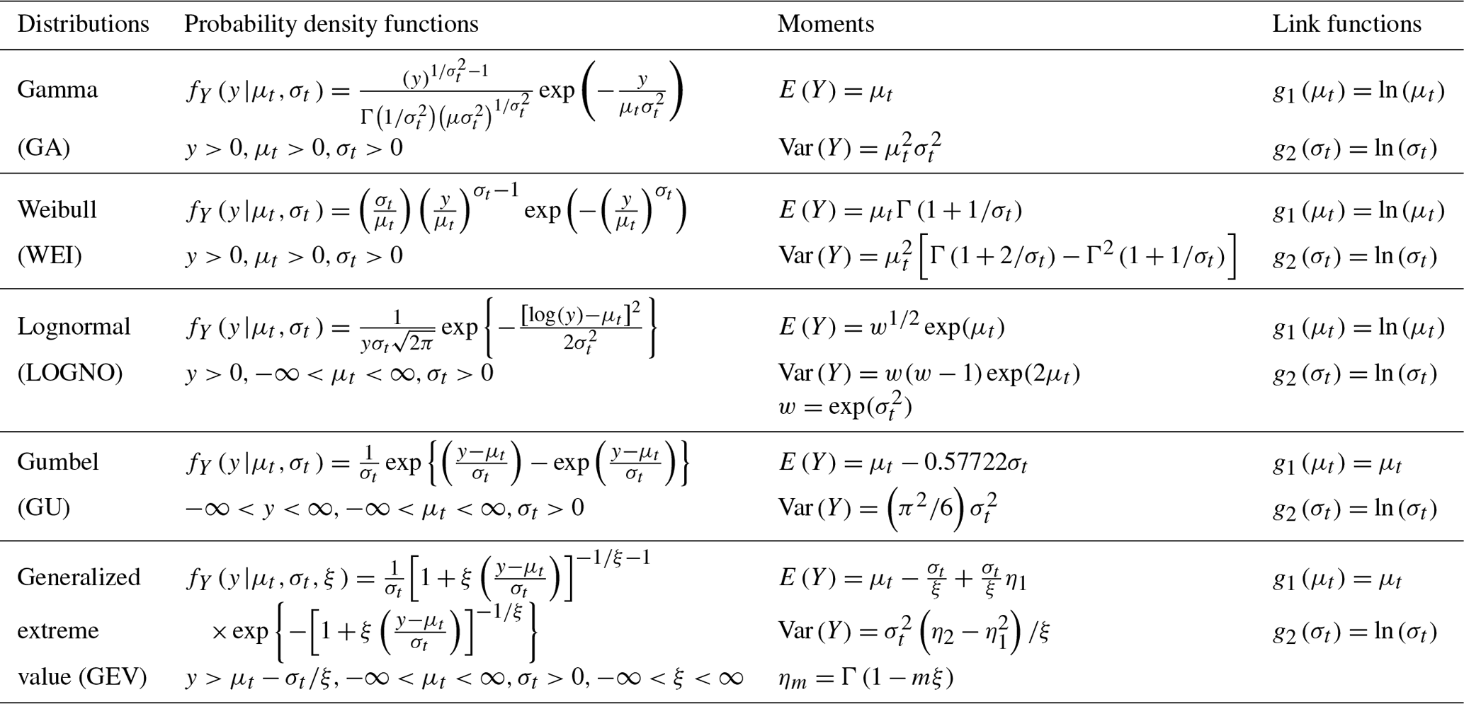
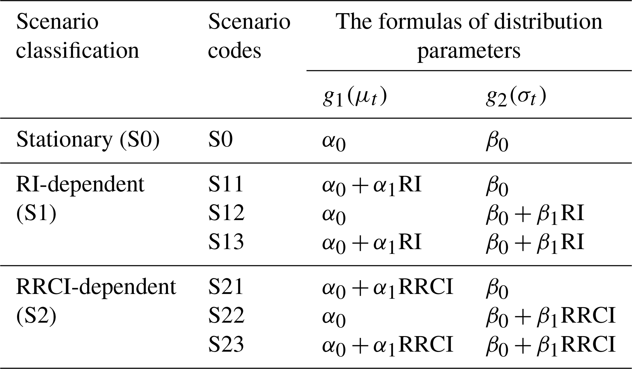
Suppose that the flood variable, Y_t, obeys the distribution $f_{Y_t}\left(y_t\left|{\mathit{\eta }}_t\right.\right)$ with the distribution parameters ${\mathit{\eta }}_t=\left[{\mathit{\mu }}_t,{\mathit{\sigma }}_t,\mathit{\xi }\right]$. In this study, only the distribution parameters μ_t and σ_t were allowed to be dependent on covariates because the shape parameter of the GEV is sensitive to the quantile estimation of rare events. According to the linear additive formulation of the generalized additive models for location, scale, and shape (GAMLSSs; Rigby and Stasinopoulos, 2005; Villarini et al., 2009), seven nonstationary scenarios for the formulas of the two distribution parameters, μ_t and σ_t, were investigated, as shown in Table 2. The constant scenario (S0) included one scenario (both μ_t and σ_t are constants). The RI-dependent scenarios (S1) included three scenarios: S11 (μ_t is RI-dependent and σ_t is constant), S12 (μ_t is constant and σ_t is RI-dependent), and S13 (both μ_t and σ_t are RI-dependent). In addition, the RRCI-dependent scenarios (S2) including S21, S22, and S23 are similar to S11, S12, and S13, respectively.

Table 2Seven nonstationary scenarios for the formulas of the two distribution parameters (i.e., μ_t and σ_t).

Download Print Version | Download XLSX

In the following, the Bayesian inference is introduced. The GEV_S23 (representing the nonstationary GEV distribution with the S23 scenario) model was used as an example, and the model parameter vector ${\mathit{\theta }}_{\mathrm{GEV}\mathrm{\_}\mathrm{S}\mathrm{23}}=\left[{\mathit{\alpha }}_{\mathrm{0}},{\mathit{\alpha }}_{\mathrm{1}},{\mathit{\beta }}_{\mathrm{0}},{\mathit{\beta }}_{\mathrm{1}},\mathit{\xi }\right]$ was used as the estimate. The Bayesian method was used to estimate θ_{GEV_S23}. Let the prior probability distribution be π(θ_{GEV_S23}) and the observations, D, have the likelihood l(D|θ_{GEV_S23}). Then the posterior probability distribution p(θ_{GEV_S23}|D) can be calculated using Bayes' theorem as follows:

where the integral is the normalizing constant, and Ω is the entire parameter space. The obvious difference between the Bayesian method and the frequentist method is that the Bayesian method considers the parameters θ_{GEV_S23} to be random variables. In addition, the desired distribution of the random variables can be obtained using a Markov chain that can be constructed using various Markov chain Monte Carlo (MCMC) algorithms (Reis and Stedinger, 2005; Ribatet et al., 2007) to process Eq. (11). In addition, in this study, the Metropolis–Hastings algorithm was used (Chib and Greenberg, 1995; Viglione et al., 2013), which was done with the aid of the R package “MHadaptive” (Chivers, 2012). A beta-distribution function was used with the parameters u=6 and v=9 , which were suggested by Martins and Stedinger (2000, 2001) as the prior distribution on the shape parameter ξ. For the other model parameters, ${\mathit{\alpha }}_{\mathrm{0}},{\mathit{\alpha }}_{\mathrm{1}},{\mathit{\beta }}_{\mathrm{0}}$ , and β₁, the prior distributions were set to non-informative (flat) priors. There are two advantages of the Bayesian method. First, as noted by El Adlouni et al. (2007), this method allows the addition of other information, such as historical and regional information, by defining the prior distribution. Second, the Bayesian method can provide an explicit way to account for the uncertainty of parameters estimates. In the nonstationary case in the t year, the 95 % credible interval for the estimation of the flood quantile corresponding to a given probability, p , can be obtained from a set of stable parameters estimations, ${\widehat{\mathit{\theta }}}_{\mathrm{GEV}\mathrm{\_}\mathrm{S}\mathrm{23}}^i$ ($i=\mathrm{1},\mathrm{2},\mathrm{\dots },M_{\mathrm{c}}$), in which M_c is the length of the Markov chain.

The procedure of model selection can identify which of the five distributions is optimal and which of the seven nonstationary scenarios is optimal. If all the distribution parameters are identified as constants (S0), this process will be a stationary frequency analysis. To select the optimal model, the Schwarz Bayesian criterion (SBC; Schwarz, 1978) for each fitted model object is calculated by the following:

where $\ln \left(\widehat{l}\right)$ is the maximized log likelihood of the model object, df is the degrees of freedom, and n is the number of data points. The SBC has a larger penalty on the overfitting phenomenon than the Akaike information criterion (AIC; Akaike, 1974). The model object with the lower SBC is preferred. The worm plot and the Q–Q plot were employed to check whether the model represented the data well.

3.1 Study area

The Han River (Fig. 4), with the coordinates of 30^∘30^′–34^∘30^′ N, 106^∘00^′–114^∘00^′ E, and a catchment area of 159 000 km², is the largest tributary of the Yangtze River, China. This area has a warm, temperate, semi-humid, continental monsoon climate. The temperature in the basin is not much different from upstream to downstream. Although the elevation range of the study area is quite wide (13–3493 m), the study area is a rainfall-dominated area, and the snowmelt contribution is quite limited. The Ankang gauging station was used as an example. The timing of the AMDF is primarily during the major rainfall period from June to September (Fig. S3a, c, and d in the Supplement). In addition, the winter is warm, with mean temperature values of more than 2 ^∘C, as shown in Fig. S3b. Since 1960, many reservoirs have been completed in the Han River basin. Information of the five major reservoirs is shown in Table 3, including the longitude, latitude, control area, time for completion, and capability. The Danjiangkou Reservoir in central China's Hubei province is the largest one in this basin and was completed by 1967. As a multi-purpose reservoir, it primarily aims to supply water and control floods, and it is also used for electricity generation and irrigation. The reservoir has a total storage capacity of 21.0 billion m³, a dead storage capacity of 7.23 billion m³, an effective storage capacity of 10.2 billion m³, and a flood control capacity of 7.72 billion m³. After the Danjiangkou Dam Extension Project in 2010, the Danjiangkou Reservoir gained an additional capacity of 13.0 billion m³ and an extra flood control storage capacity of 3.3 billion m³. In addition, this reservoir is operated using the strategy of staged increases in the flood limit water level during the flood control season (Zhang et al., 2009).

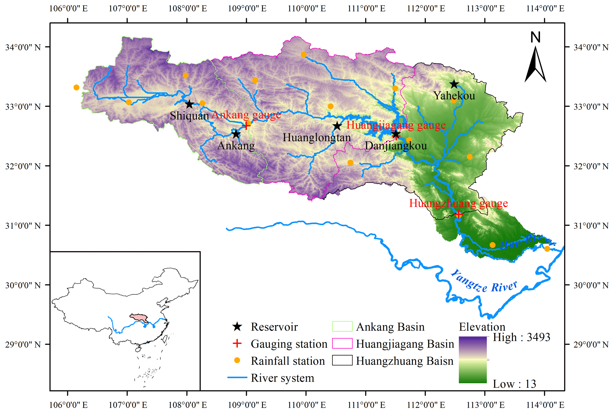
Figure 4Geographic location of the reservoirs, gauging stations, and rainfall stations along the Han River.

Table 3Information of the five major reservoirs in the Han River basin.

Download Print Version | Download XLSX

3.2 Data

The assessment analysis of reservoir effects on flood frequency utilized streamflow data, reservoir data, and rainfall data. The AMDF series was extracted from the daily streamflow records of the three gauges in the Han River basin; namely the Ankang (AK) station with a drainage area of 38 600 km², the Huangjiagang (HJG) station with a drainage area of 90 491 km², and the Huangzhuang (HZ) station with a drainage area of 142 056 km². The streamflow and reservoir data were provided by the Hydrology Bureau of the Changjiang Water Resources Commission, China (http://www.cjh.com.cn/en/index.html, last access: 9 August 2019). The annual series of the maximum (M), the intensity (I), volume (V), the timing (T), and the distance (L) were extracted from the daily streamflow data to describe the MARI. Note that the timing of the MARI is equal to the occurrence time of the AMDF during the year. The MARI is an event averaged for the real values, and any 2 consecutive days of areal rainfall values in the MARI required more than 0.2 mm. Daily areal rainfall was calculated using the inverse distance weighting (IDW) method based on rainfall records from 16 stations (shown in Fig. 4). These rainfall data were downloaded from the National Climate Center of the China Meteorological Administration (source: http://www.cma.gov.cn/, last access: 9 August 2019). For the AK and HZ gauging stations, all the records were available from 1956 to 2015, while the HJG gauging station only had records available that were from 1956 to 2013.

4.1 Identification of reservoir effects

To confirm the impact of reservoirs on the AMDF in the study area, the mean and standard deviation of the AMDF before and after the construction of the two large reservoirs, the Danjiangkou Reservoir (1967) upstream of the HJG and HZ stations and the Ankang Reservoir (1992) upstream of the AK, HJG, and HZ stations, were compared. According to Table 4, the mean and standard deviation of the AMDF of the AK, HJG, and HZ stations were significantly reduced. By using the HJG station as an example, the mean of the AMDF (1992–2013) is 4139 m³ s⁻¹, which is only 0.28 times 14 951 m³ s⁻¹ (1956–1966), and the standard deviation is 4074 m³ s⁻¹, approximately 0.52 times 7896 m³ s⁻¹ (1956–1966).

Table 4Change in the mean and standard deviation of the AMDF after the construction of the two large reservoirs (Danjiangkou Reservoir, completed by 1967, and the Ankang Reservoir, finished by 1992).

Download Print Version | Download XLSX

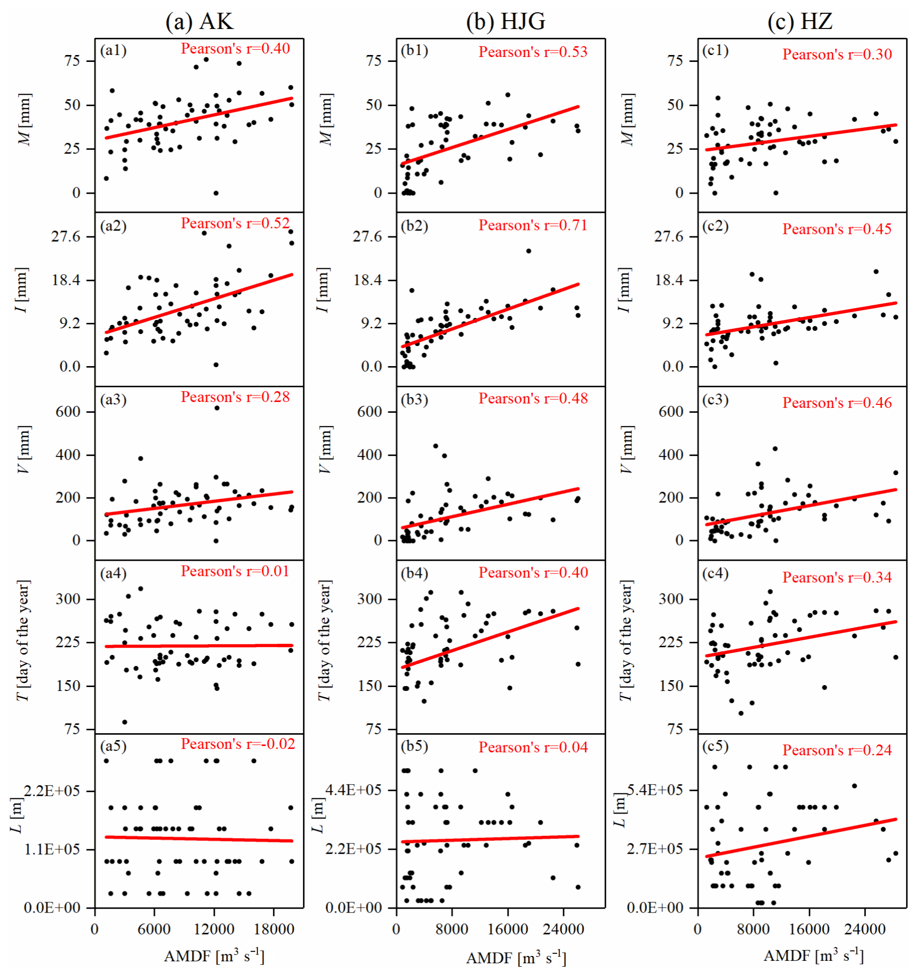
Figure 5Linear correlation between the five MARI variables and the AMDF for (a) the AK station, (b) the HJG station, and (c) the HZ station.

Download

Figure 5 presents the linear correlation between the five MARI variables (i.e., the maximum, M; the intensity, I; volume, V; the timing, T; and the distance L) and the AMDF. It was found that for M, I, V, and T, except for T in the AK station, the Pearson correlation coefficients between these four variables and the AMDF range from 0.27 to 0.71 (p value <0.05), indicating that these four variables are significantly related to the AMDF. However, there is a Pearson correlation coefficient of no more than 0.24 between L and the AMDF for each of the stations. Thus, L was excluded from the calculation of the RRCI. A further analysis of the reservoir effects on the downstream AMDF will be performed in the following sections.

4.2 Results for the rainfall–reservoir composite index (RRCI)

To obtain the annual values of the RRCI, the RI was estimated first. The RI was affected by the loss of the reservoir capacity but not to a great extent (Fig. S2). This happened because the main reservoirs (Danjiangkou and Ankang reservoirs) had a small loss rate of no more than 15 % (Table S1 and Fig. S1).

Table 5Correlation coefficients between the RRCI and the AMDF. The values in bold font are the highest absolute values of Pearson, Kendall, or Spearman correlation coefficient for the station.

^∗ The values in the first row are the correlation coefficients between RI and flood series.

Download Print Version | Download XLSX

The C-vine copula model was applied to calculate the OR-JEP of the scheduling-related MARI variables. In the modeling of the univariate marginal, the marginals of the intensity (I) of the AK and the HJG stations and the volume (V) of the HJG station were revised to deal with their significant change points (Table S2). To identify the scheduling-related variables from M, I, V, and T, the RRCI for all the possible subsets of M, I, V, and T was calculated and compared. The Pearson, Kendall, and Spearman correlation coefficients between the RRCI and the AMDF are listed in Table 5. Note that the entire decomposition structure of the C-vine copula for each RRCI of the same station was determined by the ordering of the variables of each subset (shown in the cells of the first column in Table 5). Figure 3 shows an example for the decomposition structure of the four-dimensional copula. As shown in the first row in Table 5, there is a negative correlation between the AMDF and the RI for each station. The values of the Pearson correlation coefficients between the AMDF and the RI for the AK, HJG, and HZ stations are −0.37, −0.55, and −0.53, respectively, demonstrating that there is a significant relation between the reservoir storage capacity and the reduction in the AMDF. For each station, with the exception of the RRCI of the one-dimensional case, the values of the Pearson, Kendall, and Spearman correlation coefficients between the RRCI and the AMDF are higher than between the RI and the AMDF. According to the highest Kendall correlation, the scheduling-related variables for the AK station were M, I, V, and T. Those for the HJG station were I and T, and those for the HZ station were I, V, and T.

Table 6Results of the copula models for scheduling-related rainfall variables.

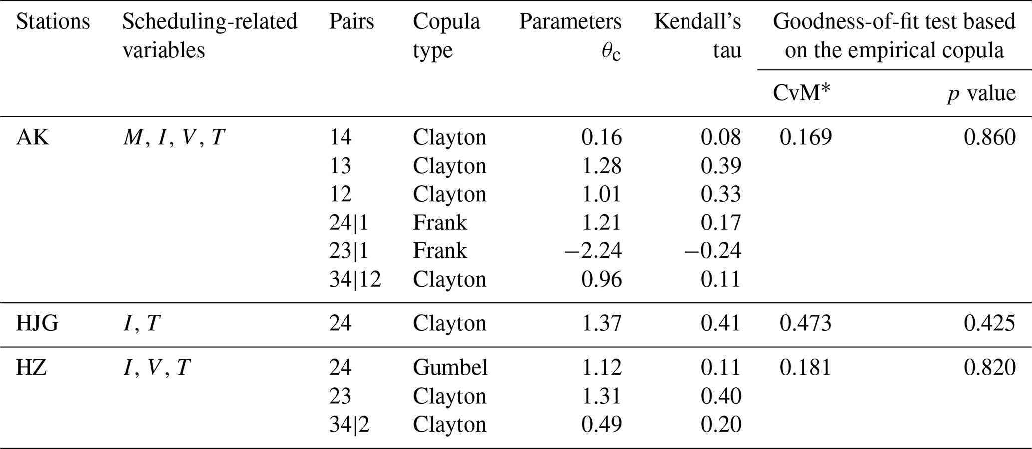
^∗ CvM is the statistic of the Cramér–von Mises test. If the p value of the C-vine copula model is less than the significance level of 0.05, the model is not considered to be consistent with the empirical copula.

Download Print Version | Download XLSX

Table 6 shows the results of the copula modeling of the scheduling-related variables using the aid of the R package “VineCopula” (https://CRAN.R-project.org/package=VineCopula, last access: 9 August 2019). Note that for each bivariate pair in the third column in Table 6, three one-parameter bivariate Archimedean copula families (i.e., the Gumbel, Frank, and Clayton copulas; Nelsen, 2007) were used to select from. As shown in Table 6, the results of the Cramér–von Mises test (Genest et al., 2009) shows that all the C-vine copula models passed the test at a significance level of 0.05. This result indicated that these models were effective for simulating the joint distribution of the scheduling-related variables for the three stations. Finally, the variation in the RI and the RRCI over time is displayed in Fig. 6. It can be seen that for each station, after reservoir construction, in most cases, the annual values of the RRCI are larger (close to 1) than those of the RI. In contrast, in a few cases, such as in 1983 at the HZ and HJG stations, the RRCI values were lower than the RI values.

Figure 6Variation of the RI and the RRCI for (a) the AK station, (b) the HJG station, and (c) the HZ station.

Download

4.3 Flood frequency analysis

A nonstationary flood frequency analysis using the RRCI or the RI as the covariate was performed to investigate how the reservoirs affected the downstream flood frequency. A summary of results of fitting the nonstationary models to the flood data is shown in Table 7. Based on the SBC, the lowest values indicate that the best models for the AK, HJG, and HZ stations are the nonstationary WEI distribution with S23, the nonstationary GA distribution with S21, and the nonstationary WEI distribution with S21, respectively, hereafter referred to as WEI_S23, GA_S21, and WEI_S21, respectively. Note that for any one of the five distributions (GA, WEI, LOGNO, GU, and GEV), the RRCI-dependent scenario had a lower SBC value than the RI-dependent scenario for each gauging station. Furthermore, for the RI-dependent and RRCI-dependent scenarios, using the HZ station as an example, the optimal formulas of the two distribution parameters, μ_t and σ_t, are given as follows:

1. WEI_S11

   $$\begin{array}{}\text{(13)}& \begin{array}{rl}& {\mathit{\mu }}_t=\exp \left(\mathrm{9.94}-\mathrm{2.79}\mathrm{RI}\right),\\ & {\mathit{\sigma }}_t=\exp \left(\mathrm{0.49}\right),\end{array}\end{array}$$

2. WEI_S21

   $$\begin{array}{}\text{(14)}& \begin{array}{rl}& {\mathit{\mu }}_t=\exp \left(\mathrm{9.92}-\mathrm{1.42}\mathrm{RRCI}\right),\\ & {\mathit{\sigma }}_t=\exp \left(\mathrm{0.73}\right).\end{array}\end{array}$$

It was found that in Eqs. (13) and (14), there were negative estimates of −2.79 and −1.42 for α₁, respectively, revealing the decreasing degree of the frequency and magnitude of downstream floods due to the reservoir effects.

Table 7Summary of the results of the nonstationary flood distribution models. The value in bold font is the lowest SBC value for the station.

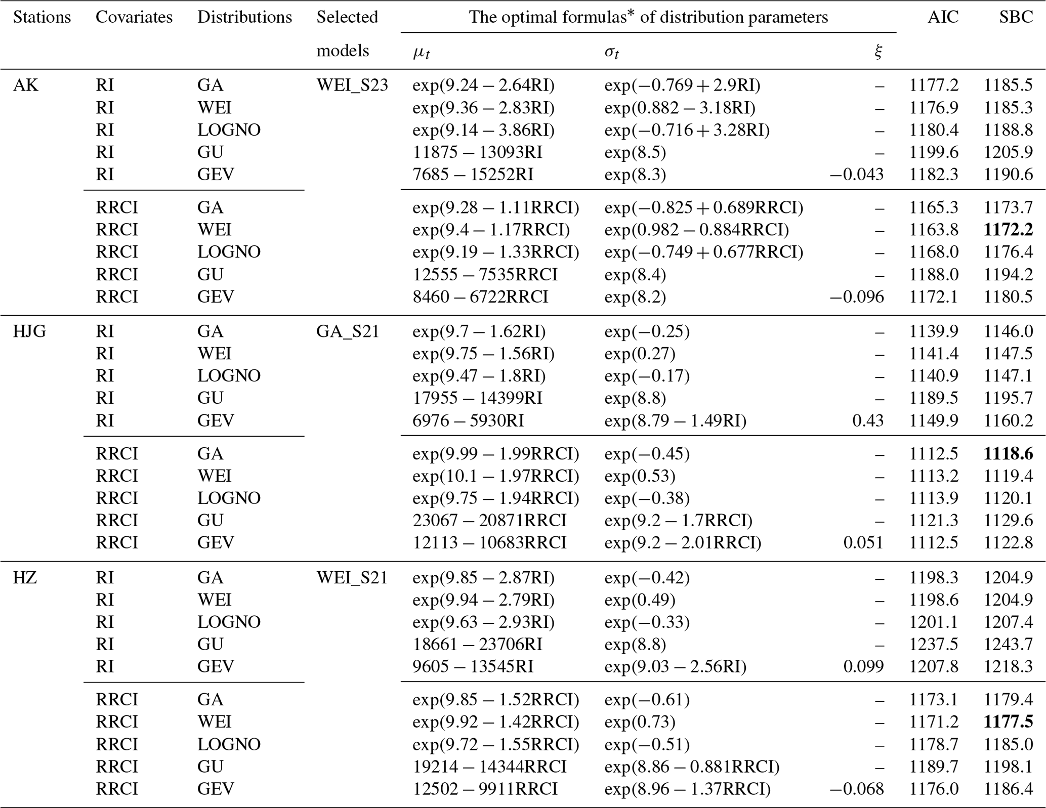
^∗ The model parameters in the optimal formulas are the posterior mean from the Bayesian inference.

Download Print Version | Download XLSX

Figure 7 compares the stationary scenario (S0), the RI-dependent scenario (S1), and the RRCI-dependent scenario (S2) of the same optimal distributions that explain all the flood values and the several largest flood values for each station. The Q–Q plots (Fig. 7a1–c1) show that overall, the RRCI-dependent scenario more adequately captured the entire empirical quantiles (particularly the smallest and largest empirical quantiles) than the two other scenarios for each station. Furthermore, as shown in Fig. 7a2–c2, for the seven largest floods (observed) of each station, the RRCI-dependent scenario produced lower quantile residuals than the two other scenarios.

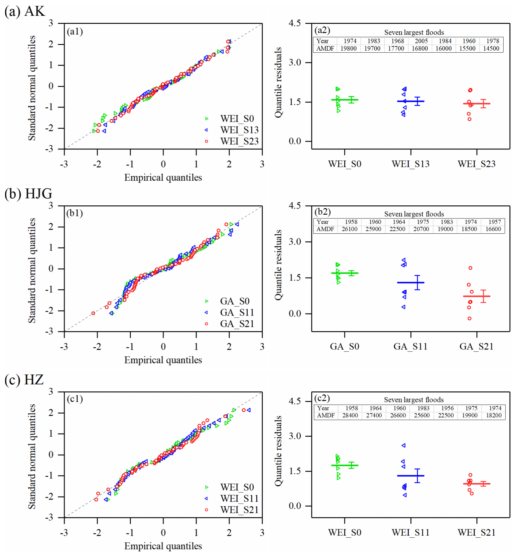
Figure 7Comparison of the stationary (S0), the RI-dependent (S1), and the RRCI-dependent (S2) scenarios of the same optimal distributions for (a) the AK station, (b) the HJG station, and (c) the HZ station. The left panels (a1, b1, c1) are the Q–Q plots for the entire AMDF series in each station. The right panels (a2, b2, c2) are the plots of the quantile residuals for the seven largest floods (their values and occurrence years have been listed) in each station, and the means of their quantile residuals (points) and the corresponding standard errors are indicated by the lines.

Download

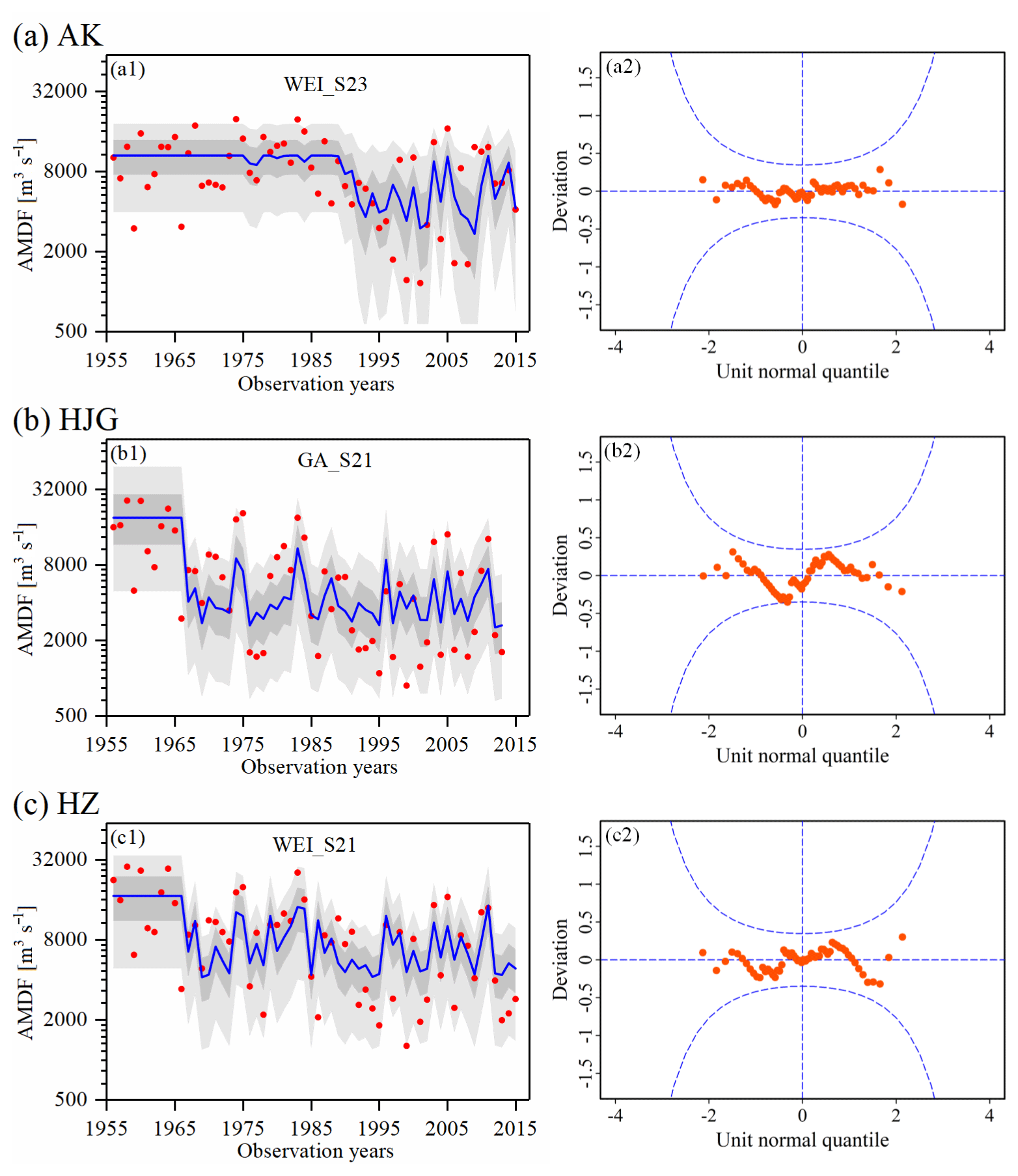
Figure 8Performance of (a) WEI_S23 for the AK station, (b) GA_S21 for the HJG station, and (c) WEI_S21 for the HZ station. The left panels (a1, b1, c1) are the centile-curve plots in each station (the 50th centile curves are indicated by the thick blue lines, the light grey-filled areas are between the 5th and 95th centile curves, the dark grey-filled areas are between the 25th and 75th centile curves, and the filled red points indicate the observed series). The right panels (a2, b2, c2) are the worm plots. In a reasonable model, the plotted points should be within the 95 % confidence intervals (between the two blue dashed curves).

Download

Figure 8 shows the performance of the best models: WEI_S23 for the AK station, GA_S21 for the HJG station, and WEI_S21 for the HZ station. The points in the worm plots in Fig. 8 are within the 95 % confidence interval, indicating that the selected models are reasonable. In addition, according to the centile-curve plots in Fig. 8, the AMDF series is well fitted by the best models. Undoubtedly, with the incorporation of the effects of the MARI, the RRCI-dependent scenario captured the presence of nonstationarity in the downstream flood frequency well. The case of the HZ station was used for the analysis (Fig. 8c1). After the construction of the Danjiangkou Reservoir (1967), due to reservoir operation, most of the values of the AMDF had been reduced in magnitude by this reservoir. However, some relatively large flood events still occurred several times, such as 25 600 m³ s⁻¹ in 1983 and 19 900 m³ s⁻¹ in 1975. Obviously, this phenomenon of flood occurrences was explained well by the RRCI.

Figure 9Statistical inference of the 100-year return levels with a 95 % uncertainty interval using the optimal RI-dependent and the RRCI-dependent distributions: (a) WEI_S13 and WEI_S23 for the AK station, (b) GA_11 and GA_S21 for the HJG station, and (c) WEI_S11 and WEI_S21 for the HZ station. In nonstationary case, the 95 % credible interval in the t year is calculated by a set of the (99th) percentile estimations, which are obtained by the flood distribution functions determined by the values of both covariate in that year and posterior parameter samples.

Download

The 100-year return levels at a 95 % credible interval from WEI_S23 and WEI_S13 for the AK station, GA_S21 and GA_S11 for the HJG station, and WEI_S21 and WEI_S11 for the HZ station are presented in Fig. 9. For each station, compared to the optimal RI-dependent distribution, the optimal RRCI-dependent distribution provided a lower 100-year return level. However, exceptions existed. In addition, after the construction of the main reservoir, the uncertainty range of the AK station was larger than that of the HJG and HZ stations. A possible explanation for the larger uncertainty range was that the sample size (1993–2015) of the regulated floods at the AK station was smaller. Furthermore, the dependent relationship between the RRCI and the AMDF at the AK station was weaker.

4.4 Discussion

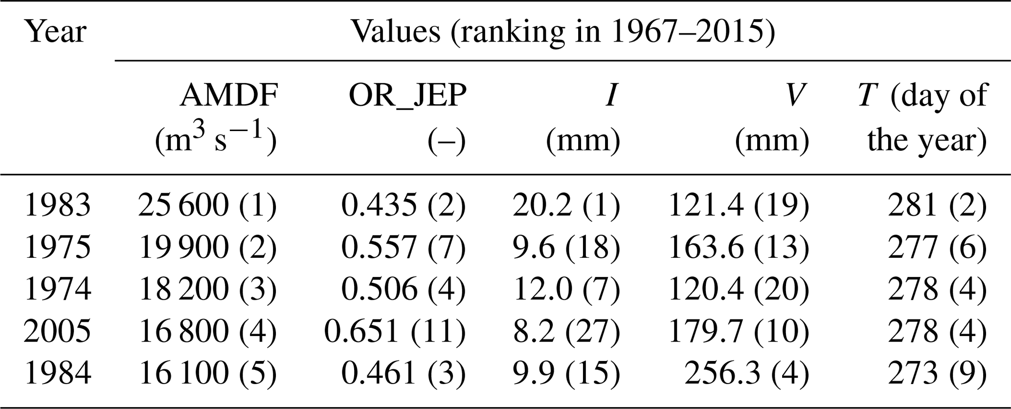
The long-term variation in the AMDF series (Fig. 8) indicates that the upstream reservoirs had evidently altered the downstream flood regimes. As an example, since the completion of the Danjiangkou Reservoir in 1967, the flood magnitude of the HZ station was evidently reduced overall. This is consistent with the results of the effects of reservoirs on the hydrological regime in this area found in previous studies (Cong et al., 2013; Guo et al., 2008; Jiang et al., 2014; Lu et al., 2009). In this study, it was found that there was a significant difference between downstream floods affected by the same reservoir system (with the same RI value). In most cases, relatively small downstream floods were obtained. However, it is of interest to note that unexpected large downstream floods still occurred in a few cases in spite of a large RI value. For example, most values of the AMDF in the HZ station have been less 10 000 m³ s⁻¹ since 1967, but the values of the AMDF in 1983 and in 1975 were 25 600 and 19 900 m³ s⁻¹, respectively. These unexpected large downstream floods were probably related to the MARI effects on reservoir operation. The five largest (unexpected) floods since 1967 and the corresponding values of the scheduling-related MARI variables in the HZ station are shown in Table 8. It was found that the largest floods from 1967 to 2015 occurred in 1983. For this flood event, the MARI was a rare event (with an OR-JEP value of 0.435 ranking second in 1967–2015) due to the largest mean intensity (I=20.2 mm) and the second latest occurrence (T=281). Surprisingly, all the timing values of the MARI for these five unexpected downstream floods showed high rankings (second to ninth). These timing values were near the end (approximately the 300th day of the year) of the flood control period (July–October) in this area. Actually, near the end of the major flood control period, the storage capacity should be decreased. This is because according to the operation rules of the Danjiangkou Reservoir (Zhang et al., 2009), there is a staged increasing flood limit water level during the flood control season. One important cause for those unexpected large downstream floods was probably that the remaining storage capacity at the end of flood season was not sufficient to reduce some late floods. Therefore, in addition to the storage capacity of reservoirs, the MARI effects should be indispensably considered when attempting to accurately quantify the effects of the reservoir on downstream floods.

Table 8Summary of the rainfall information for the five largest floods after the construction (1967) of the Danjiangkou Reservoir in the HZ station.

Download Print Version | Download XLSX

With the combination of both the RI and the OR-JEP, the RRCI had a significant difference from RI (Fig. 6). With a few exceptions, the RRCI values were higher than the RI values. This indicates that the real reservoir impact may be underestimated by the RI in most cases. Moreover, the RI will also probably overestimate the real reservoir impact in a few cases because of not considering special rainfall events (i.e., the MARI with low values of the OR-JEP). The results of the covariate-based nonstationary flood frequency analysis (Table 7 and Figs. 7 and 8) demonstrate that, compared to the RI-dependent scenario, the RRCI-dependent scenario for the optimal nonstationary distribution more completely captured the presence of nonstationarity in the downstream flood frequency. Therefore, the RRCI might be a useful index for accessing the reservoir effects on downstream flood frequency.

Finally, the estimation errors of the OR-JEP should be noted. (1) Only those MARI samples that corresponded to the timing of the AMDF were included to estimate the OR-JEP. This means that some extreme MARI samples that corresponded to the non-maximum flow were not included, resulting in an estimation error for the OR-JEP. To reduce this error, it might be worth considering the use of the peaks-over-threshold sampling method. (2) The areal-averaged MARI was based on the records from 16 rainfall stations using the IDW method. The estimation error of the areal-averaged rainfall can be transferred to the OR-JEP estimation error. Additional rainfall site data and spatial distribution information were needed to reduce the OR-JEP estimation error. Nonetheless, the good performance of the downstream flood frequency model results demonstrated that the MARI samples still remained representative in this study.