the Creative Commons Attribution 4.0 License.
the Creative Commons Attribution 4.0 License.
 | 30 Oct 2019
Future shifts in extreme flow regimes in Alpine regions
Manuela I. Brunner
Daniel Farinotti
Harry Zekollari
Matthias Huss
Massimiliano Zappa
Extreme low and high flows can have negative economic, social, and ecological effects and are expected to become more severe in many regions due to climate change. Besides low and high flows, the whole flow regime, i.e., annual hydrograph comprised of monthly mean flows, is subject to changes. Knowledge on future changes in flow regimes is important since regimes contain information on both extremes and conditions prior to the dry and wet seasons. Changes in individual low- and high-flow characteristics as well as flow regimes under mean conditions have been thoroughly studied. In contrast, little is known about changes in extreme flow regimes. We here propose two methods for the estimation of extreme flow regimes and apply them to simulated discharge time series for future climate conditions in Switzerland. The first method relies on frequency analysis performed on annual flow duration curves. The second approach performs frequency analysis of the discharge sums of a large set of stochastically generated annual hydrographs. Both approaches were found to produce similar 100-year regime estimates when applied to a data set of 19 hydrological regions in Switzerland. Our results show that changes in both extreme low- and high-flow regimes for rainfall-dominated regions are distinct from those in melt-dominated regions. In rainfall-dominated regions, the minimum discharge of low-flow regimes decreases by up to 50 %, whilst the reduction is 25 % for high-flow regimes. In contrast, the maximum discharge of low- and high-flow regimes increases by up to 50 %. In melt-dominated regions, the changes point in the other direction than those in rainfall-dominated regions. The minimum and maximum discharges of extreme regimes increase by up to 100 % and decrease by less than 50 %, respectively. Our findings provide guidance in water resource planning and management and the extreme regime estimates are a valuable basis for climate impact studies.
Highlights
-
Estimation of 100-year low- and high-flow regimes using annual flow duration curves and stochastically simulated discharge time series
-
Both mean and extreme regimes will change under future climate conditions.
-
The minimum discharge of extreme regimes will decrease in rainfall-dominated regions but increase in melt-dominated regions.
-
The maximum discharge of extreme regimes will increase and decrease in rainfall-dominated and melt-dominated regions, respectively.


Low flows can have severe impacts on ecology and economy. Potential ecological impacts include fish-habitat conditions or water quality (Rolls et al., 2012), whilst economical impacts comprise water supply, river transport, agriculture, and energy production (Van Loon, 2015). The intensity of such potentially harmful low flows is projected to increase in the future due to climate change (Alderlieste et al., 2014; Papadimitriou et al., 2016; Marx et al., 2018). Also, high flows, which can cause severe damages and major costs (Aon Benfield, 2016), are expected to change in future. While clear patterns of change have been detected for flood timing (Blöschl et al., 2017), changes in magnitude are less clear than for low flows (Madsen et al., 2014). Together with low and high flows, the whole flow regime, which depicts the magnitude, variability, and seasonality of discharge during the year (Poff et al., 1997), is expected to change (Arnell, 1999; Horton et al., 2006; Laghari et al., 2012; Addor et al., 2014; Milano et al., 2015). Such changes are caused by reduced snow and glacier storage (Beniston et al., 2018), related reductions in melt contributions (Farinotti et al., 2016; Jenicek et al., 2018), and changes in precipitation seasonality and intensity (Brönnimann et al., 2018). It is important to quantify these hydrological changes to adapt water governance and management accordingly (Clarvis et al., 2014).
Previous studies have focused on the detection of changes in mean flow regimes (Horton et al., 2006; Addor et al., 2014; Milano et al., 2015). For planning purposes and river basin management, however, estimates not only for mean conditions, but also for extreme conditions, are needed (Van Loon, 2015; Ternynck et al., 2016). Extreme regime estimates, which describe the evolution of flow over the year under extreme conditions, provide guidance for water managers, decision makers, and engineers involved in planning and water management. They are essential for the adaptation of hydraulic infrastructure such as reservoirs and for developing suitable water management and flood protection strategies.
Commonly, extreme flow estimates derived by frequency analysis focus on one characteristic of the hydrological regime, e.g., summer low flows, drought durations, drought deficits (e.g., Tallaksen, 2000; WMO, 2008), flood peaks, or flood volumes (e.g., Mediero et al., 2010; Brunner et al., 2017). The focus on one or several of these individual characteristics, however, neglects the pre-conditions of low- and high-flow events. However, for low-flow events, these pre-conditions are crucial for the formation of groundwater storage (Şen, 2015), reservoir filling (Hänggi and Weingartner, 2012; Anghileri et al., 2016), and soil moisture formation (Zampieri et al., 2009). These storages can become very important when it comes to the satisfaction of diverse water needs and to the alleviation of water shortages (Mussá et al., 2015; Brunner et al., 2019b). In the case of high flows, antecedent conditions determine the proportion of rainfall transformed to direct runoff and therefore the severity of the flood event (Berghuijs et al., 2016; Nied et al., 2017). In contrast to the individual low- and high-flow characteristics, the flow regime includes information on both the pre-conditions and the discharge during the low- and high-flow seasons.
Estimating extreme flow regimes with a given exceedance frequency is not straightforward since discharge values at several points in time are correlated. Because of the multivariate nature of the problem, no single solution exists. We here aim at estimating extreme high- and low-flow regimes with a defined return period for current and future climate conditions. We propose two possible approaches for the estimation of such extreme regimes. The first approach is based on flow duration curves (FDCs). FDCs describe the whole distribution of discharge and are particularly suited for planning purposes (Vogel and Fennessey, 1994; Claps and Fiorentino, 1997). It has been shown that frequency analysis performed on annual FDCs allows for the estimation of extreme FDCs with pre-defined return periods (Castellarin et al., 2004; Iacobellis, 2008). While such estimates contain information on the frequency of occurrence and the distribution of flow, they lack information on the seasonality of flow (Vogel and Fennessey, 1994). FDC estimates derived for a certain return period T therefore need to be recombined with a specific seasonality, e.g., the long-term one. This first estimation approach treats distribution and seasonality separately. To overcome this problem, an alternative approach based on stochastically generated time series is proposed. Stochastically generated time series have been used in a number of water resource studies, including hydrologic design and drought planning (Koutsoyiannis, 2000). Stochastic approaches generate large sets of realizations of possible discharge time series, thus sampling hydrologic variability beyond the historical record (Herman et al., 2016; Tsoukalas et al., 2018), potentially including extreme events and regimes. In hydrology, stochastic models have been developed so as to reproduce key statistical features of observed data, including the distribution and the temporal dependence (Sharma et al., 1997; Salas and Lee, 2010; Tsoukalas et al., 2018).
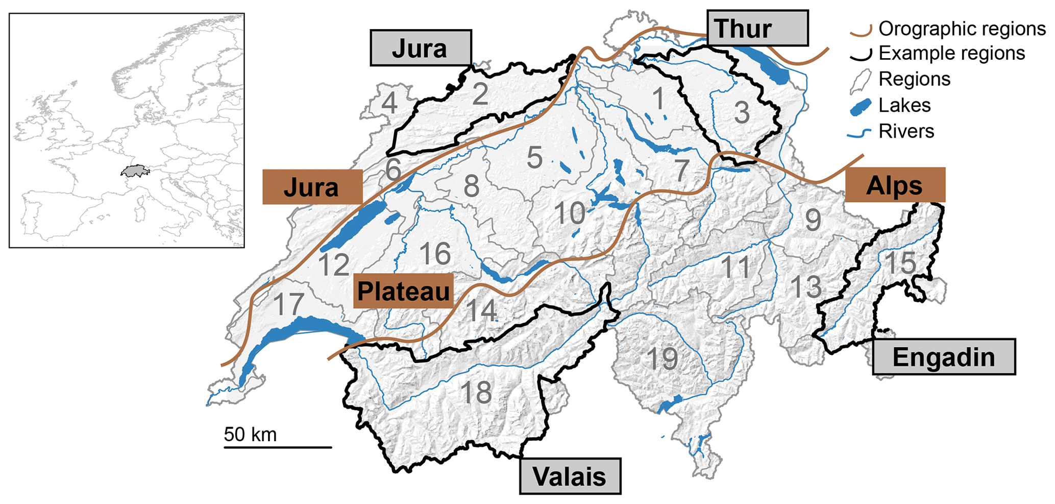
Figure 1Map of Switzerland with 19 large hydrological regions (grey outline) and the four illustration regions (black border): Thur, Jura, Valais, and Engadin. The main orographic regions Jura, Plateau, and Alps are outlined by the brown lines.
Many different approaches have been proposed for the stochastic simulation of streamflow time series. Often, indirect approaches, which combine the stochastic simulation of rainfall with hydrological models, have been used for the generation of stochastic discharge time series (Pender et al., 2015). These approaches are affected by uncertainties due to hydrological model selection and calibration, which can be avoided by using direct synthetic streamflow generation approaches (Herman et al., 2016). Direct approaches stochastically simulate discharge. The simplest types of models to describe daily streamflow are autoregressive moving average (ARMA) models (Pender et al., 2015; Tsoukalas et al., 2018). However, this type of model only captures short-range dependence (Koutsoyiannis, 2000). Models also capturing long-range dependence include fractional Gaussian noise models (Mandelbrot, 1965), fast fractional Gaussian noise models (Mandelbrot, 1971), broken line models (Mejia et al., 1972), and fractional autoregressive integrated moving average models (Hosking, 1984). Alternatives to these time-domain models are frequency-domain models (Shumway and Stoffer, 2017). These latter use phase randomization to simulate surrogate data with the same Fourier spectra as the raw data (Theiler et al., 1992; Radziejewski et al., 2000). Despite their favorable characteristics, such methods based on the Fourier transform have been rarely applied in hydrology (Fleming et al., 2002). We apply the approach of phase randomization to simulate stochastic discharge time series using the approach proposed by Brunner et al. (2019a) (provided in the R-package PRSim, which can be found in the CRAN repository https://cran.r-project.org/web/packages/PRSim/index.html approaches, last access: 7 October 2019). As opposed to classical phase randomization, this approach does not rely on the empirical distribution, but uses the flexible, four-parameter kappa distribution (Hosking, 1994), which allows for the generation of a wide range of realizations of high and low discharge values. Among these simulated series, extreme regimes can be identified. After having identified a suitable approach for the estimation of extreme regimes, we apply this approach to discharge time series representing future climate conditions. A comparison to current estimates allows us to identify future changes in extreme high- and low-flow regimes.
2.1 Study area
The analyses were performed on a set of 19 hydrological regions in Switzerland (Fig. 1) with areas between 600 and 5000 km2, mean elevations between 550 and 2300 m a.s.l., and mean annual precipitation sums between 1000 and 1800 mm. The flow regimes north of the Alps (Plateau and Jura) are dominated by rainfall and characterized by high discharge in winter and spring but low discharge in summer. In contrast, the regimes in the Alps are dominated by snowmelt and ice melt and characterized by high discharge in summer. For illustration purposes, we chose four regions. Two of them (Jura and Thur) have a rainfall-dominated regime and the other two (Valais and Engadin) a melt-dominated regime under the current climate.
2.2 Analysis framework
The analysis performed to detect changes in future extreme regimes consisted of three main steps (Fig. 2). First, different procedures for estimating extreme flow regimes were tested (first step). Once a suitable procedure was identified, it was applied to estimate extreme high- and low-flow regimes under current and future climate conditions (second step). These extreme regimes were compared to mean regimes. Third, current and future estimates were compared to detect future changes in flow regimes (third step). We used simulated discharge representing both current and future climatology as the basis for the analysis. The current discharge series were derived by feeding a hydrological model with observed meteorological data and with meteorological data simulated by a set of climate models for the reference period. The future discharge series were obtained by driving the model with meteorological data from downscaled and bias-corrected climate model simulations.
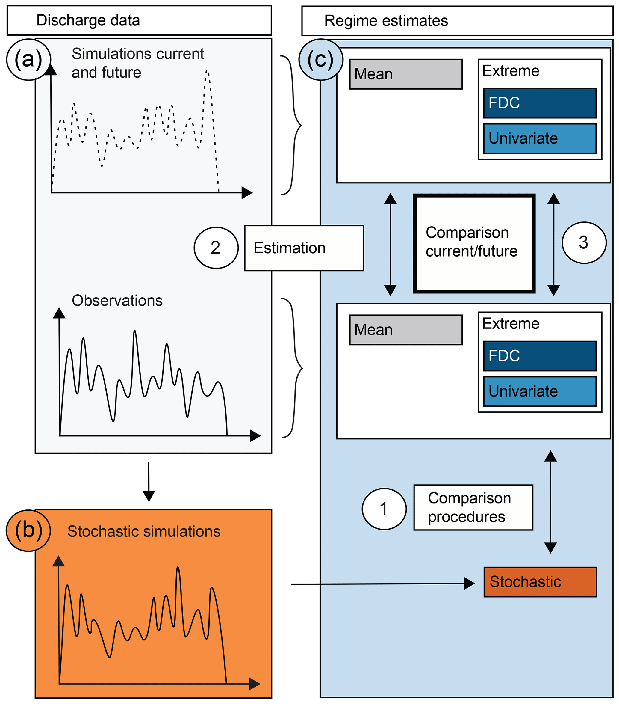
Figure 2Illustration of the study framework. (1) Comparison of the different estimation techniques univariate, FDC, and stochastic, (2) estimation of current and future mean and extreme regimes using simulated discharge time series, and (3) comparison of current and future regime estimates. The paper (a) introduces the simulated data used, (b) outlines the stochastic discharge generator, and (c) describes the estimation approaches.
The two estimation techniques applied use frequency analysis of different quantities. The first method applies frequency analysis to the individual percentiles of the FDC. The second method uses stochastically simulated discharge time series to identify annual hydrographs with a certain non-exceedance probability. We refer to these methods as FDC and stochastic, respectively. The two methods are compared to a benchmark method (univariate), which performs univariate frequency analysis of the monthly discharge values and neglects the dependence between individual months. We here focus on the estimation of high- and low-flow regimes with a return period of T=100 years since this return period is commonly used for planning purposes. The methods outlined in this study, however, can be generalized to other return periods. In the following paragraphs, we describe the data sets (Fig. 2a, Sect. 2.3), the stochastic discharge generation procedure (Fig. 2b, Sect. 2.4), and the estimation techniques used to derive extreme flow regimes (Fig. 2c, Sect. 2.5).
2.3 Hydrological simulations
We used discharge time series simulated with the PREVAH hydrological model (Viviroli et al., 2009b) as input for the analysis. To represent current conditions, the model was driven with observed meteorological data for the period 1981–2010. To represent future conditions, it was driven with meteorological data obtained by regional climate model simulations for the period 2071–2100 (see below). PREVAH is a conceptual process-based model. It consists of several sub-models representing different parts of the hydrological cycle: interception storage, soil water storage and depletion by evapotranspiration, groundwater, snow accumulation and snowmelt and glacier melt, runoff and baseflow generation, plus discharge concentration and flow routing (Viviroli et al., 2009b). A gridded version of the model at a spatial resolution of 200 m was set up for Switzerland (Speich et al., 2015). For the calibration of the model parameters, meteorological and discharge time series from 140 mesoscale catchments covering different runoff regimes were used. The model calibration was conducted over the period 1993–1997. Validation on discharge was performed with the period 1983–2005. More details on the calibration and validation procedures can be found in Köplin et al. (2010). The parameters for each model grid cell were derived by regionalizing the parameters obtained for the 140 catchments with ordinary kriging (Viviroli et al., 2009a; Köplin et al., 2010). The hydrological model has been calibrated using observed meteorological data, but will subsequently be fed with meteorological data simulated by a set of GCM–RCM combinations. It is assumed that the parameter set derived in the calibration procedure will still produce reliable results since Krysanova et al. (2018) have confirmed in a review that a good performance of hydrological models in the historical period increases confidence in projected impacts under climate change. Future glacier extents were simulated with two glacier evolution models. We used the global glacier evolution model (GloGEM; Huss and Hock, 2015) for short glaciers (glacier length < 1 km) and GloGEMflow (Zekollari et al., 2019) for long glaciers (length > 1 km). GloGEM simulates glacier changes with a retreat parameterization relying on observed glacier changes (Huss et al., 2010). GloGEMflow is an extended version of GloGEM with a dynamic ice flow component. This new model was extensively validated over the European Alps through comparisons with various observations (e.g., surface velocities and observed glacier changes) and detailed 3-D projections from modeling studies focusing on individual glaciers (e.g., Jouvet et al., 2011; Zekollari et al., 2014). The simulated glacier extents were transformed from the GloGEM(flow) 1-D model grid to the 2-D PREVAH model grid by ensuring that the area for each elevation band was conserved.
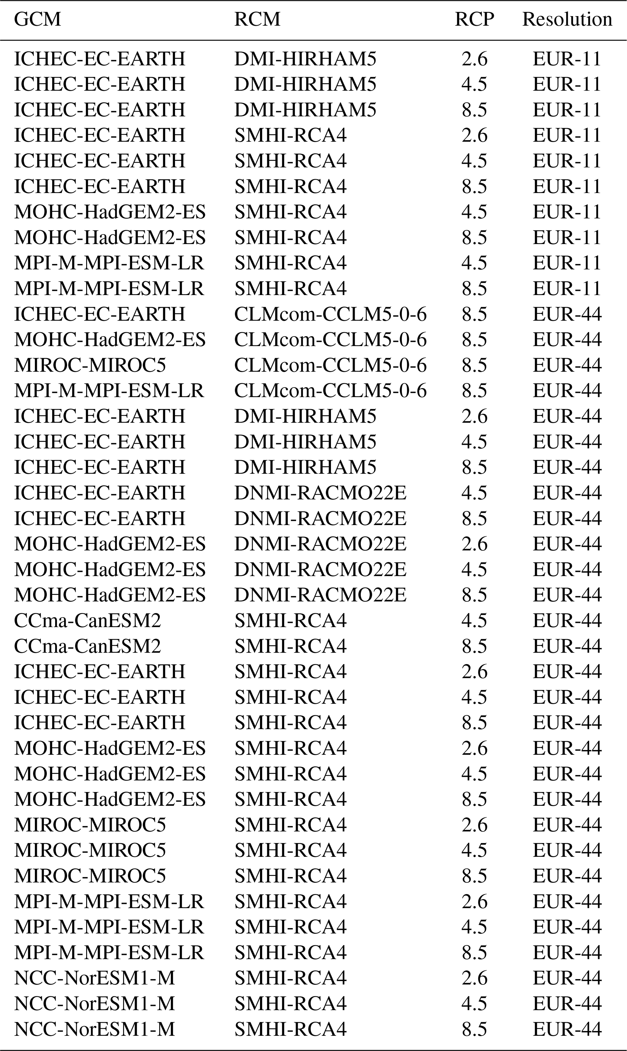
PREVAH is driven by time series of precipitation, temperature, relative humidity, shortwave radiation, and wind speed. The meteorological forcing for current simulations was observed time series provided by the Federal Office of Meteorology and Climatology MeteoSwiss (2018), while the transient meteorological forcing for future simulations was derived from the CH2018 climate scenarios (National Centre for Climate Services, 2018). The meteorological data were interpolated to a 2×2 km grid using detrended inverse distance weighting where the detrending was based on a regression between climate variables and elevation (Viviroli et al., 2009b). The climate scenarios are based on the results from the EURO-CORDEX initiative (Jacob et al., 2014; Kotlarski et al., 2014), which are the most sophisticated and high-resolution coordinated climate simulations over Europe. The scenarios are based on representative concentration pathways (RCPs) (Moss et al., 2010; Meinshausen et al., 2011; van Vuuren et al., 2011) and a regional downscaling approach based on quantile mapping (Themeßl et al., 2012; Gudmundsson et al., 2012). The quantile mapping procedure was calibrated on the period 1981–2010 and performed on a grid-by-grid basis for all meteorological variables. The meteorological data were derived from an ensemble of 39 GCM–RCM combinations for different scenarios (Table A1 in the Appendix), which provide temperature, precipitation, relative humidity, shortwave radiation, and wind speed for the locations of various meteorological stations. The selection of scenarios included the three RCPs2.6, 4.5, and 8.5 for which 8, 13, and 18 GCM–RCM combinations were available, respectively. Ten out of the 39 GCM–RCM combinations were available at a high resolution of 12.5 km and the remaining combinations at a resolution of roughly 50 km. Using combinations at both resolutions allows for a larger ensemble; however, it means that those GCM–RCM combinations which are available for both resolutions obtain more weight. During a model run, PREVAH reads the meteorological grids and further downscales the data to the computational grid of 200×200 m using bilinear interpolation. For temperature, a lapse rate of −0.65 ∘C/100 m was additionally used for topographic corrections.
2.4 Stochastic simulation of discharge time series
The discharge simulated with the hydrological model for the current (1981–2010) and future (2071–2100) 30-year periods only represents small sets of possible annual hydrograph realizations. Among these realizations, certain hydrographs including extreme hydrographs such as a 100-year hydrograph were possibly not observed. We used a stochastic discharge simulation procedure to increase the number of possible annual hydrograph realizations. These realizations represent the discharge statistics and temporal correlation structure of the available data and extend the existing sample to as yet unobserved annual hydrographs. To simulate such hydrographs, we used the method of phase randomization (Theiler et al., 1992; Schreiber and Schmitz, 2000). We combined this empirical procedure with the flexible four-parameter kappa distribution (Hosking, 1994) to allow for the extrapolation to as yet unobserved values. This phase randomization approach preserves the autocorrelation structure of the raw series by conserving its power spectrum (Theiler et al., 1992). The procedure consists of three main steps (Radziejewski et al., 2000). In a first step, the discharge series (here, the simulated discharge for past and future conditions) is converted from the time domain to the spectral domain by the Fourier transform (Morrison, 1994). The Fourier transform of a given time series x=(x1, …, xt, …, xn) of length n is
where t is the time step, ω are the phases, and is the imaginary unit. In this spectral domain, the data are represented by the phase angle and by the amplitudes of the power spectrum as represented by the periodogram. The phase angle of the power spectrum is uniformly distributed over the range −π to π. In a second step, the phases in the phase spectrum are randomized, while the power spectrum is preserved. In a third step, the inverse Fourier transform is applied to transform the data from the spectral domain back to the temporal domain. A step-by-step description of the stochastic simulation procedure and more background information on the Fourier transform are provided in Brunner et al. (2019a), and references therein. An application of the simulation procedure to four example catchments in Switzerland has shown that both seasonal statistics and temporal correlation structures of discharge can be well reproduced (Brunner et al., 2019a). We therefore used this method to stochastically simulate 1500 years of discharge for each of the 19 regions in our data set. Stochastic series representing current conditions were generated by using the hydrological model simulations for 1981–2010 obtained by the 39 GCM–RCM combinations as input. Stochastic series representing future conditions were generated based on each of the hydrological model simulations generated with the 39 GCM–RCM combinations for different scenarios.
2.5 Estimation of T-year hydrographs
We employed two methods for estimating 100-year low- and high-flow regimes: FDC and stochastic. The extreme regime estimates were compared to the stochastically generated hydrographs to check for plausibility. Furthermore, they were compared to a lower-bound (for low-flow regimes) or upper-bound (for high-flow regimes) benchmark regime derived by combining 100-year monthly discharge estimates obtained from univariate frequency analysis. This frequency analysis was performed on the values of each month independently and the monthly values were fitted with a generalized extreme value (GEV) distribution. This distribution was not rejected according to the Anderson–Darling goodness-of-fit test computed using the procedure proposed by Chen and Balakrishnan (1995) (α=0.05). The disadvantage of the univariate procedure is that the autocorrelation in the data, which is mainly visible for lags of 1 and 2 months, is neglected, which overestimates the extremeness of the 100-year low-flow regime and therefore produces unrealistic estimates. The univariate approach will therefore only be considered as a benchmark for model comparison and will not find consideration in the comparison of current and future extreme regime estimates.
2.5.1 FDC
A first extreme regime estimate was derived by performing the frequency analysis of annual FDCs. According to Vogel and Fennessey (1994), an annual FDC with an assigned return period can be obtained from the pth quantile function. To do so, we fitted a GEV distribution to the quantiles corresponding to each percentile. The GEV was not rejected based on the Anderson–Darling goodness-of-fit test (α=0.05). The fitted GEV distributions were used to estimate the 100-year quantile for each percentile. The 100-year FDC was then derived by combining these 100-year quantiles. The 100-year FDC does not contain any information about the seasonality, but only about the statistical distribution of flow. To include information about seasonality, we combined the estimated 100-year FDC with a typical seasonal regime. To do so, the individual quantile values of the FDC were assigned to the corresponding ranks of a typical flow regime. This typical regime was defined as the long-term (mean) regime of the daily input time series and varied for current and future conditions. The estimated extreme discharge regimes were aggregated to a monthly resolution to make them comparable to the univariate estimates.
2.5.2 Stochastic
The second method for the estimation of extreme regimes performs the frequency analysis directly on a large set of stochastically simulated annual hydrographs (here 1500 years). The frequency analysis was performed on the annual sums of the stochastically generated hydrographs. We identified the hydrograph corresponding to the empirical 100-year annual discharge sum as the 100-year regime. The application of this procedure is only possible for long time series as given by the stochastic series, since a 100-year annual sum is not necessarily observed in a short record of, say, 30 years. Like the FDC estimates, the regimes derived from the stochastic approach were aggregated to a monthly resolution.
2.6 Comparison of current and future regime estimates
The two methods and the benchmark approach for the estimation of 100-year low- and high-flow regime estimates were applied to discharge time series representing current and future climate conditions. First, 100-year regimes were estimated for current conditions (1981–2010). To generate a control regime, we used the discharge simulated with the observed meteorological data. To represent uncertainty due to different GCM–RCM combinations for different scenarios, we derived one reference regime for each discharge time series simulated by the 39 climate GCM–RCM combinations for different scenarios. This analysis provided us with a range of current regime estimates due to climate model uncertainty. The regime estimates derived from the 39 GCM–RCM combinations were used to derive a multi-model mean, which served as a reference for determining changes between current and future conditions. In a second step, 100-year estimates were derived for future conditions using the simulated time series for the period 2071–2100 for all GCM–RCM combinations and scenarios. We assessed changes in seasonality and magnitude of flow regimes in terms of their minimum, maximum, and mean discharges by comparing regime estimates derived for future conditions to the multi-model mean representing current conditions. (Figure 3; results were grouped by RCP.)
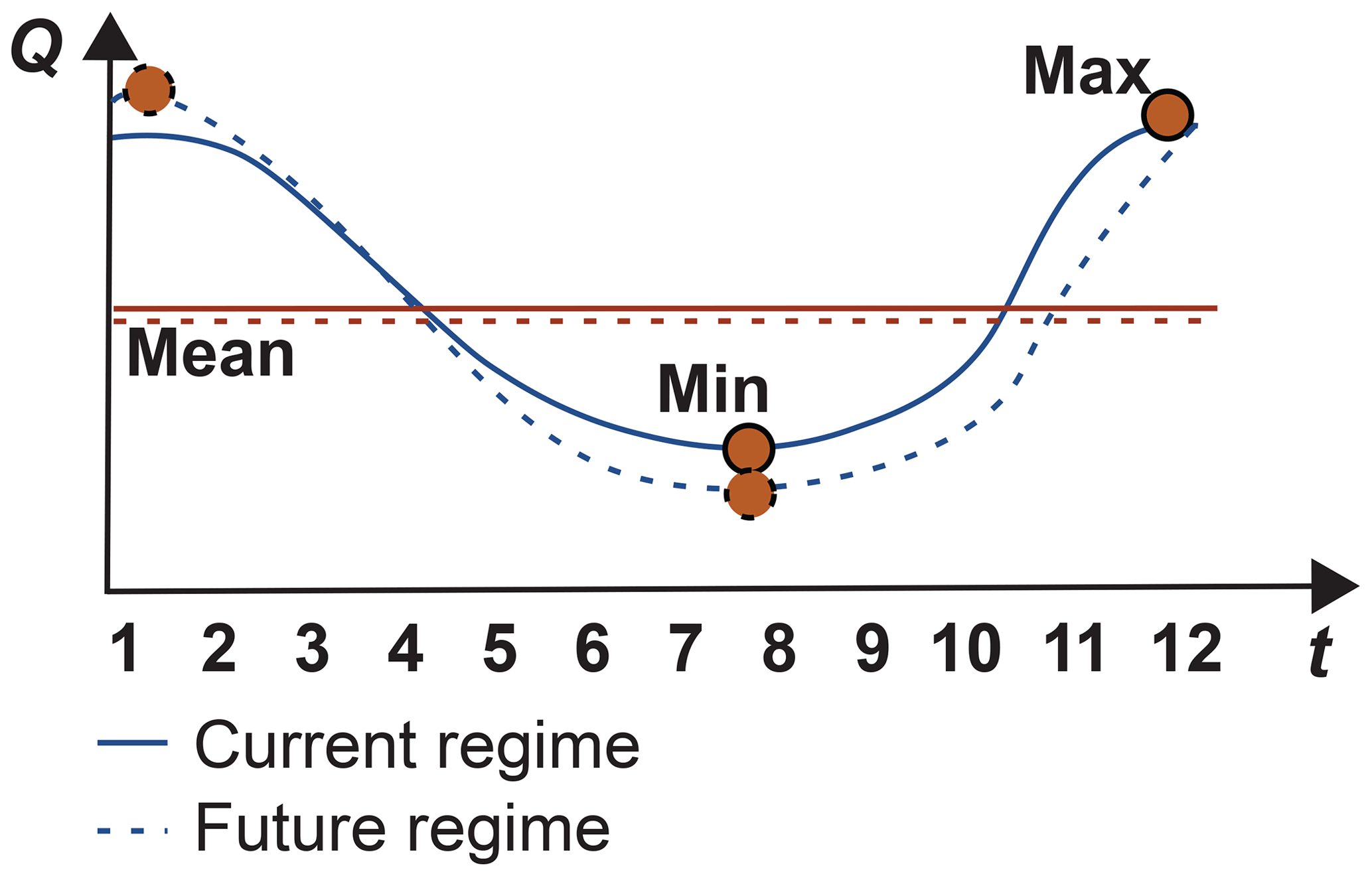
Figure 3Illustration of the main characteristics of an annual rainfall-dominated flow regime under current and future conditions: maximum, mean, and minimum.
3.1 Comparison of estimation methods
The two estimation techniques and the benchmark approach provide distinct estimates for the 100-year low-flow regimes (Fig. 4). The univariate technique leads to the most extreme regimes, whilst the FDC and stochastic methods lead to similar estimates. The univariate estimate should only be seen as a lower benchmark and not as an estimate for a “true” 100-year regime since the univariate approach neglects the dependence between monthly estimates. In contrast, the FDC and stochastic approaches produce more plausible estimates, i.e., estimates at the lower bound of the observed values. The summer low-flow regimes estimated by the FDC technique are comparable to the regimes of the year 2003, which included a very dry summer (Beniston, 2004; Rebetez et al., 2006; Schär et al., 2004; Zappa and Kan, 2007).
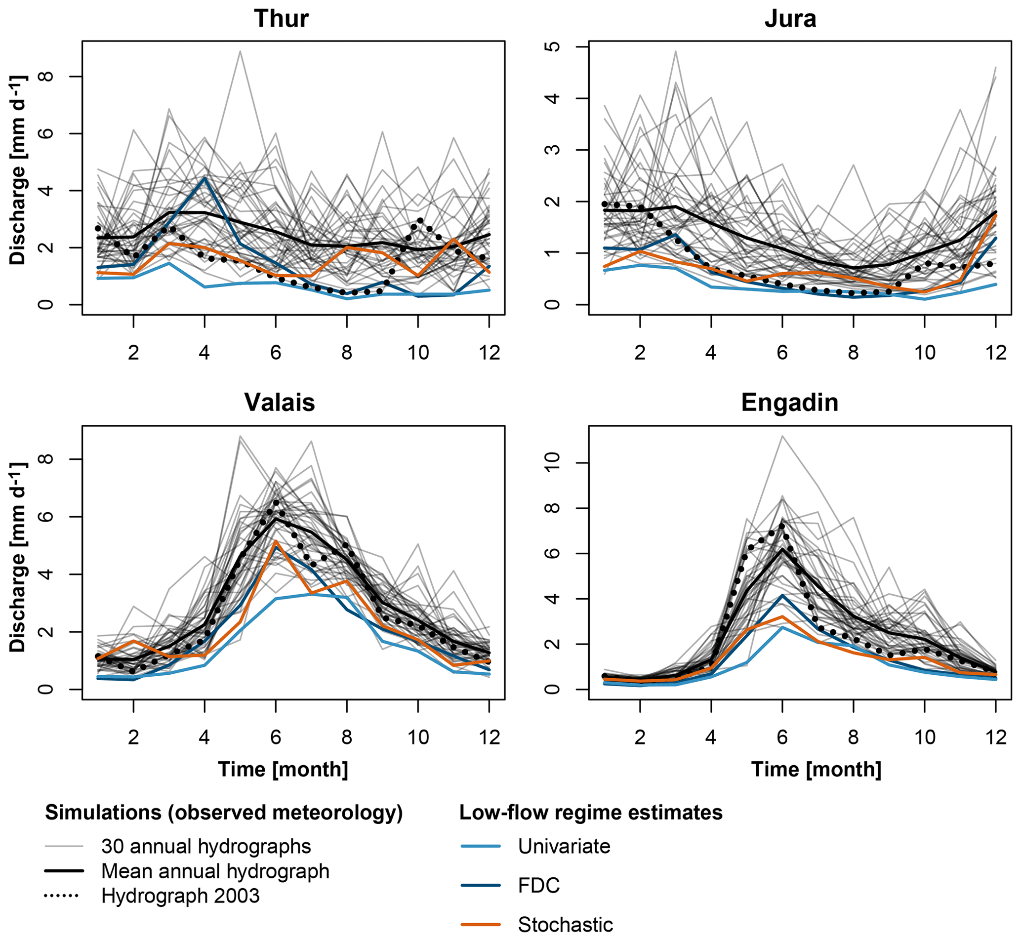
Figure 4100-year low-flow regime estimates for current climate conditions (control) derived using univariate frequency analysis (light blue), frequency analysis of the FDC (dark blue), and stochastically generated time series (orange). The annual hydrographs simulated using observed meteorological data are given in grey, while the mean annual hydrograph and the hydrograph simulated for the year 2003 are given in black. The four panels are shown on different scales.
Similarly to low-flow regimes, the 100-year high-flow regimes derived by the three estimation techniques are distinct (Fig. 5). The univariate approach, as mentioned previously, produces unrealistic results in terms of seasonality, since the predictions of the monthly 100-year flows neglect the dependence between the different months. The FDC and stochastic techniques produce more similar seasonalities and more realistic estimates at the upper bound of the observed annual hydrographs. Contrary to low-flow estimates, high-flow estimates generated with the FDC or stochastic techniques can be different. The stochastic approach generally leads to more conservative estimates than the FDC approach in melt-dominated regions. We attribute this to the fact that the stochastic approach performs frequency analysis of annual sums, while the FDC approach performs frequency analysis of the percentiles of the FDC.
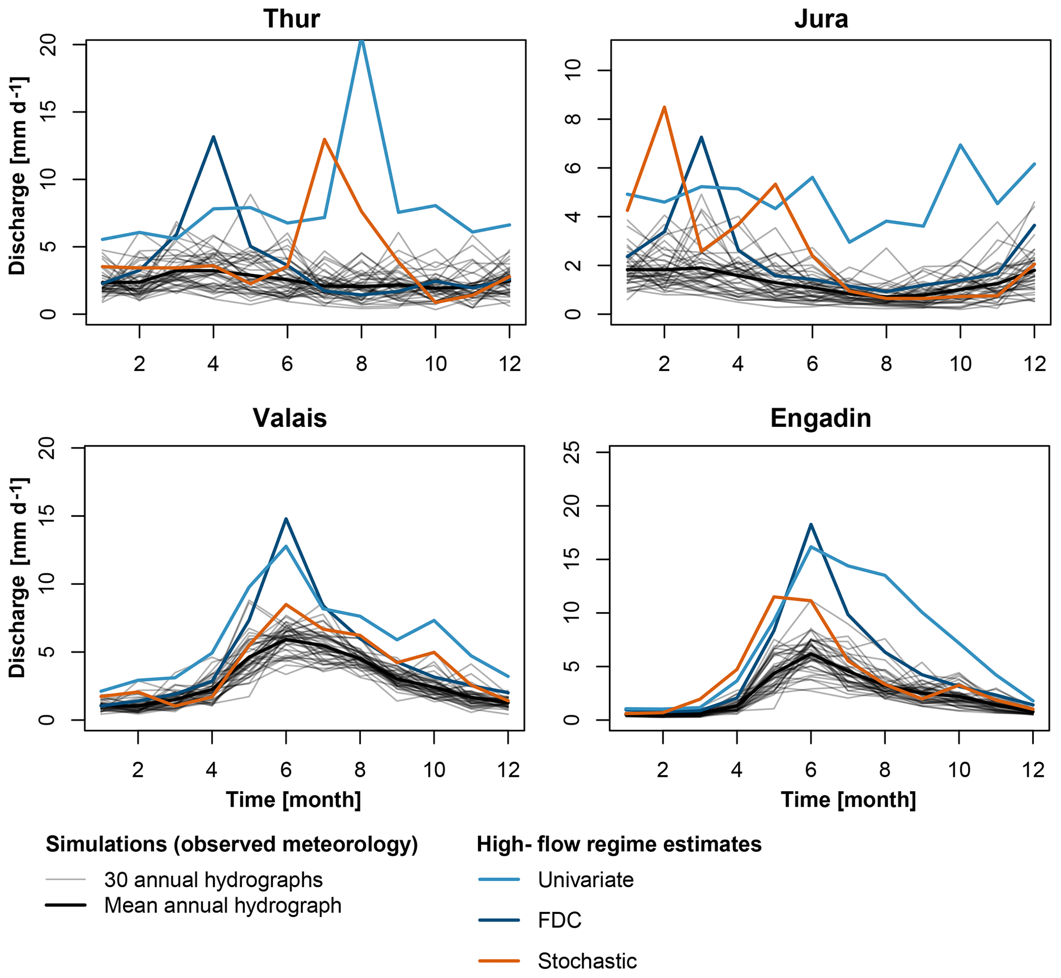
Figure 5100-year high-flow regime estimates for current conditions (control) derived using univariate frequency analysis (light blue), frequency analysis of the FDC (dark blue), and stochastically generated time series (orange). The annual hydrographs simulated using observed meteorological data are given in grey, while the mean annual hydrograph is given in black. The four panels are shown on different scales.
The plausibility of the 100-year estimates derived by using the FDC and stochastic approaches is shown by a comparison with stochastically generated annual hydrographs (Fig. A1 in the Appendix for the low-flow estimates). The derived estimates, in fact, are embedded in the lower spectrum of the stochastically generated annual hydrographs. This is hardly the case for the univariate estimates, which lead to “unrealistically low” 100-year hydrographs partly outside of the range of the stochastically generated hydrographs. Similarly, the 100-year high-flow regime estimates derived by the FDC and stochastic methods are embedded in the higher spectrum of the stochastically generated hydrographs, while the univariate estimate is “unrealistically high”. Since the univariate approach yields unrealistic estimates, it is not considered for further analysis.
3.2 Current and future low-flow regime estimates
Both mean and extreme regimes are subject to uncertainty when derived from simulated discharge. The uncertainty comes from the hydrological model and from the spread between the climate simulations. Figure 6 shows mean and extreme low- and high-flow regime estimates derived for the observed climatology for the four illustration catchments. It also shows the range of regimes obtained by using different GCM–RCM combinations and scenarios. This range of regimes generally encompasses the regime derived from meteorological observations, which suggests that the climate model output realistically reproduces the observed climate. An exception is the Engadin, where the low-flow regimes derived from the GCM–RCM combinations overestimate summer low flows. This overestimation might be related to the univariate bias correction applied, which might not perfectly reflect the interplay between temperature and precipitation and therefore the timing of snowmelt processes (Meyer et al., 2019). The spread in the current regimes is larger for extreme than for mean conditions for the rainfall-dominated catchments Thur and Jura. In addition, the spread is larger for the high- than for the low-flow extreme regimes except for the Engadin region. This range should be kept in mind when analyzing future regime estimates.
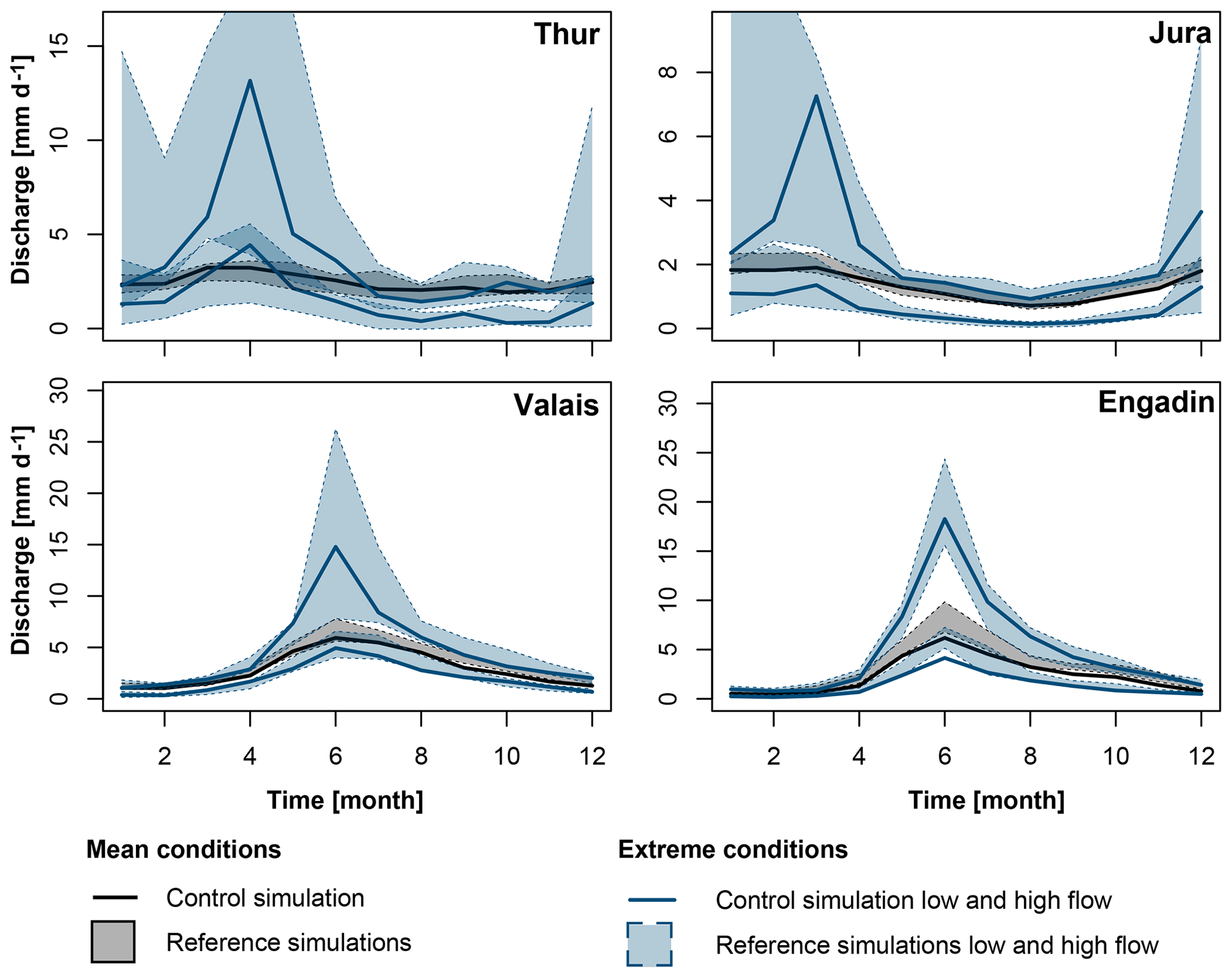
Figure 6Current 100-year mean regimes (grey), low-flow regimes (blue lower line), and high-flow regimes (blue upper line) estimated by using the FDC method on the control discharge simulations derived by observed meteorological data (bold line) and the reference discharge simulations derived by meteorological data simulated by the 39 GCM–RCM combinations for different scenarios for the reference period (shaded polygons).
Shifts in regimes are expected for both mean and extreme low-flow conditions (Fig. 7). The shifts are weak for rainfall-dominated regions (e.g., Thur and Jura), while they are strong for melt-dominated regions (e.g., Valais and Engadin). For the rainfall-dominated regions, changes in mean and extreme regimes are most visible for RCP8.5. Here, the different realizations lead to regimes with more pronounced summer low flows. In addition, there is a reduction in spring discharge under RCP2.6 for both mean and extreme conditions when looking at the regimes derived from the FDC approach. In the case of melt-dominated regions, most GCM–RCM combinations lead to clear shifts towards regimes with earlier and reduced summer flows. These shifts are more pronounced for RCP8.5 than RCPs4.5 and 2.6. Note that the spread of future regimes is smaller for RCP2.6 than RCPs4.5 and 8.5 due to the smaller number of chains in the ensemble.

Figure 7Comparison of current multi-model mean (solid line) and future 100-year low-flow regime estimates (shaded polygons) over the 39 GCM–RCM combinations and scenarios derived by the FDC (blue) and stochastic (orange) approaches. The mean regimes are provided as a reference (grey).
Differences between current (i.e., multi-model mean of reference simulations) and future mean and extreme low-flow regimes are summarized in Fig. 8. The detected changes for RCP2.6 and RCP8.5 are similar (results for RCP4.5 are not displayed, but lie in between those of RCPs2.6 and 8.5). Changes are projected for the minimum and maximum discharges of mean and extreme low-flow regimes and for their timing, but less for the mean of these regimes. The changes in the mean flow can reach up to 30 %, while the maximum and minimum flows can change up to 100 %.
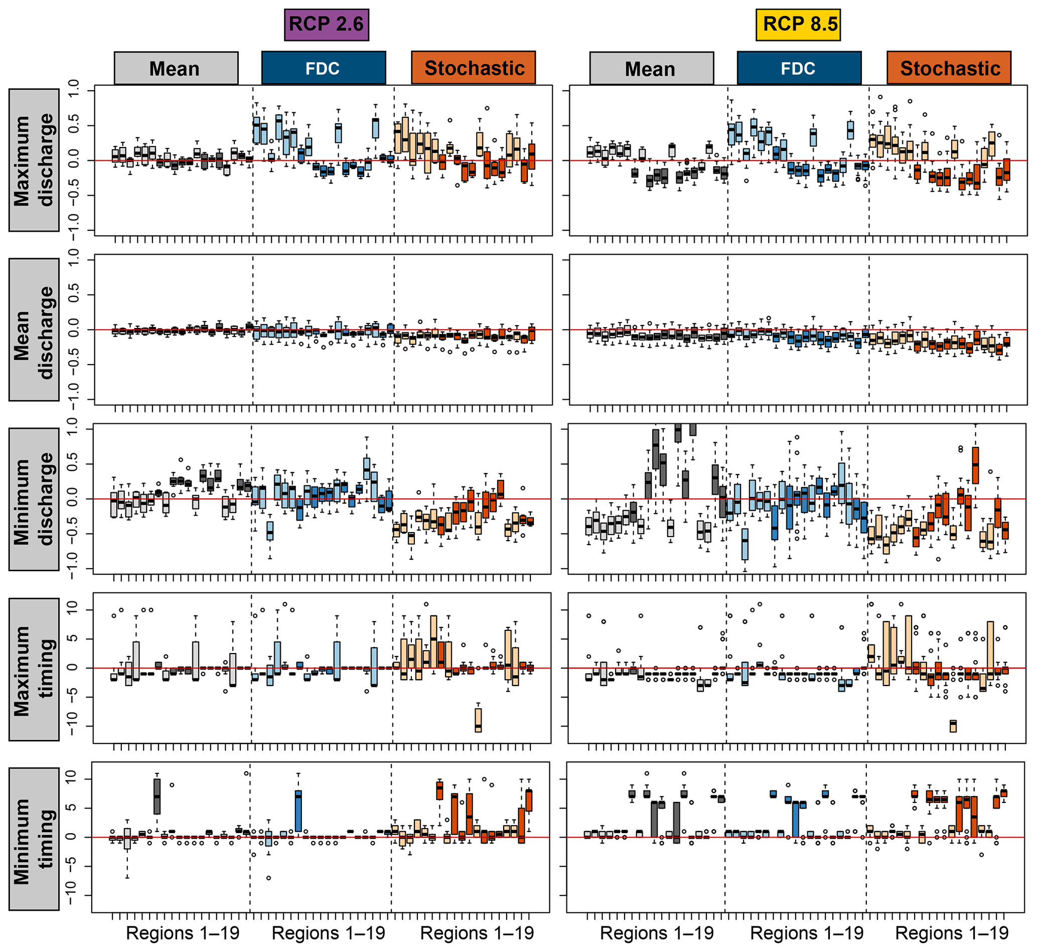
Figure 8Differences between current (i.e., multi-model mean of reference simulations) and future mean (grey) and extreme low-flow regime characteristics for the 19 regions (Fig. 1) estimated by the FDC (blue) and stochastic (orange) approaches. Five indicators are shown: maximum discharge, mean discharge, minimum discharge, timing of minimum discharge, and timing of maximum discharge. The first three rows show relative changes, the last two rows changes in months. Melt-dominated (dark colors) and rainfall-dominated regions (light colors) are distinguished. The boxplots indicate the range resulting from using the 39 GCM–RCM combinations for different scenarios.
Changes in melt- and rainfall-dominated regions are clearly different. Both the FDC and stochastic approach suggest changes in extreme low-flow regimes. In rainfall-dominated regions, an increase is expected for the discharge maximum independent of the estimation approach chosen. In contrast, a decrease is expected in the discharge minimum according to the stochastic approach, while no clear changes are expected using the FDC approach. For melt-dominated regions, the change pattern is different. There, a decrease in maximum discharge is expected. An increase in minimum discharge is expected for mean regimes, while changes are less clear for the extreme regimes. Shifts of 1 or 2 months are expected in timing for both rainfall- and melt-dominated regions. In most catchments, the timing of future maximum discharge is likely to occur earlier than under current conditions. Shifts towards later in the year are expected in the timing of the minimum flow. The changes in mean and maximum flows are similar for extreme low-flow regimes derived by the two estimation techniques FDC and stochastic. In contrast, the shifts in minimum flow and timing are different when applying the stochastic approach instead of the FDC approach.
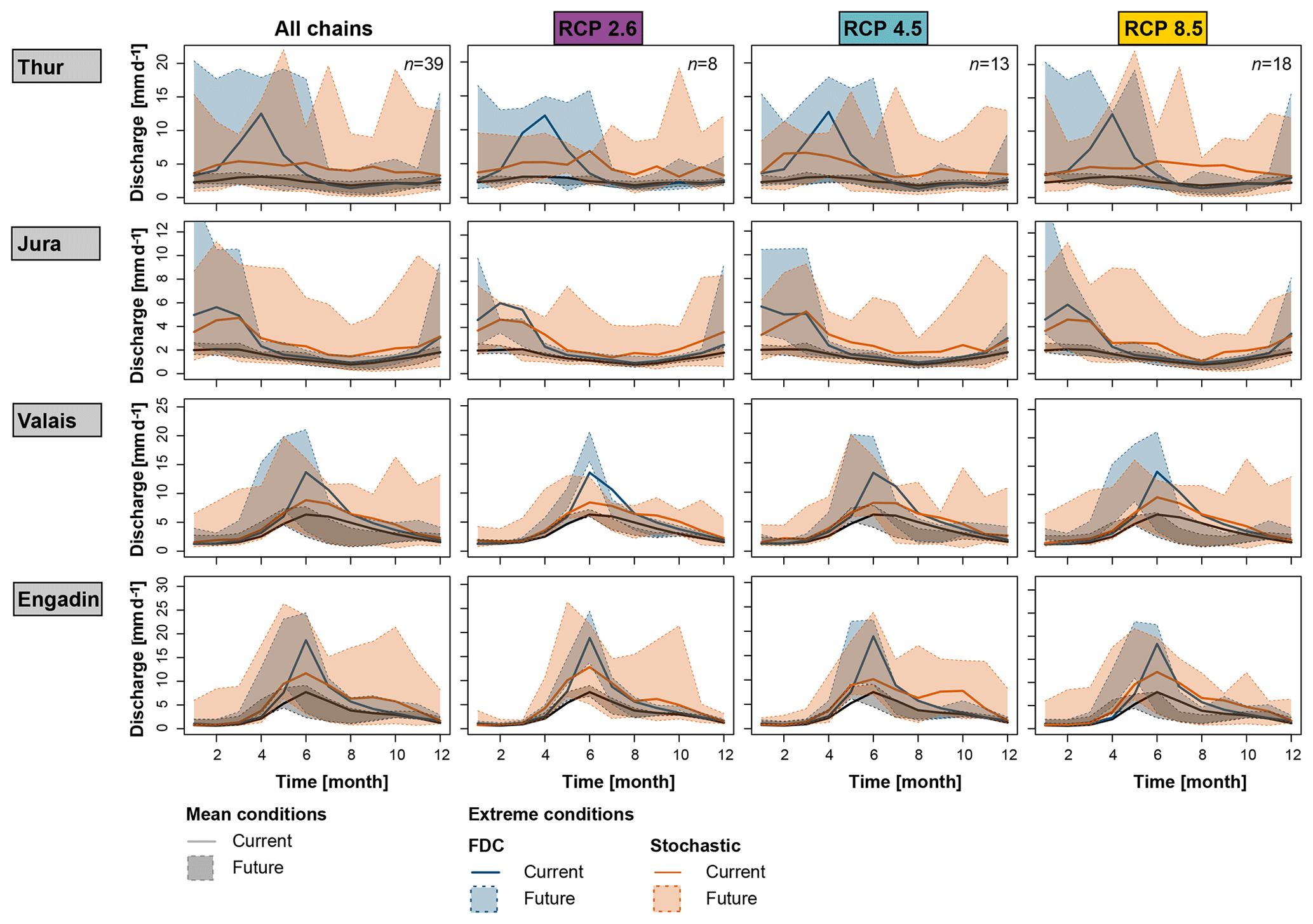
Figure 9Comparison of current multi-model mean (solid line) and future 100-year high-flow regime estimates (shaded polygons) over the 39 GCM–RCM combinations derived by the FDC (blue) and stochastic (orange) approaches. The mean regimes are provided as a reference (grey).
3.3 Current and future high-flow regime estimates
High-flow regime estimates are also expected to change (Fig. 9), with no consistent change pattern visible at first glance. Changes in high-flow extreme regimes are slightly more pronounced for RCP8.5 than for RCP2.6 (Fig. 10; RCP4.5 not shown because it is expected to provide results somewhere in between RCPs2.6 and 8.5). They are similar for the estimation techniques used (FDC/stochastic). As for the low-flow regimes, only moderate and mostly positive changes of less than 30 % are expected in the mean discharge of extreme high-flow regimes. The changes in the maximum and minimum discharges of the high-flow regimes are much stronger, i.e., up to 100 %. In rainfall-dominated regions, changes in maximum discharge are mostly positive, while they can be negative for melt-dominated regions. In these melt-dominated regions, an increase is expected in the minimum discharge of high-flow extreme regimes, especially when using the FDC approach. In rainfall-dominated regions, changes in minimum discharge are mostly negative, especially for RCP8.5. Changes in timing are different for the FDC and stochastic approach and there is no consistent pattern across catchments. Minimum and maximum discharges can occur earlier or later in the year than under current conditions.
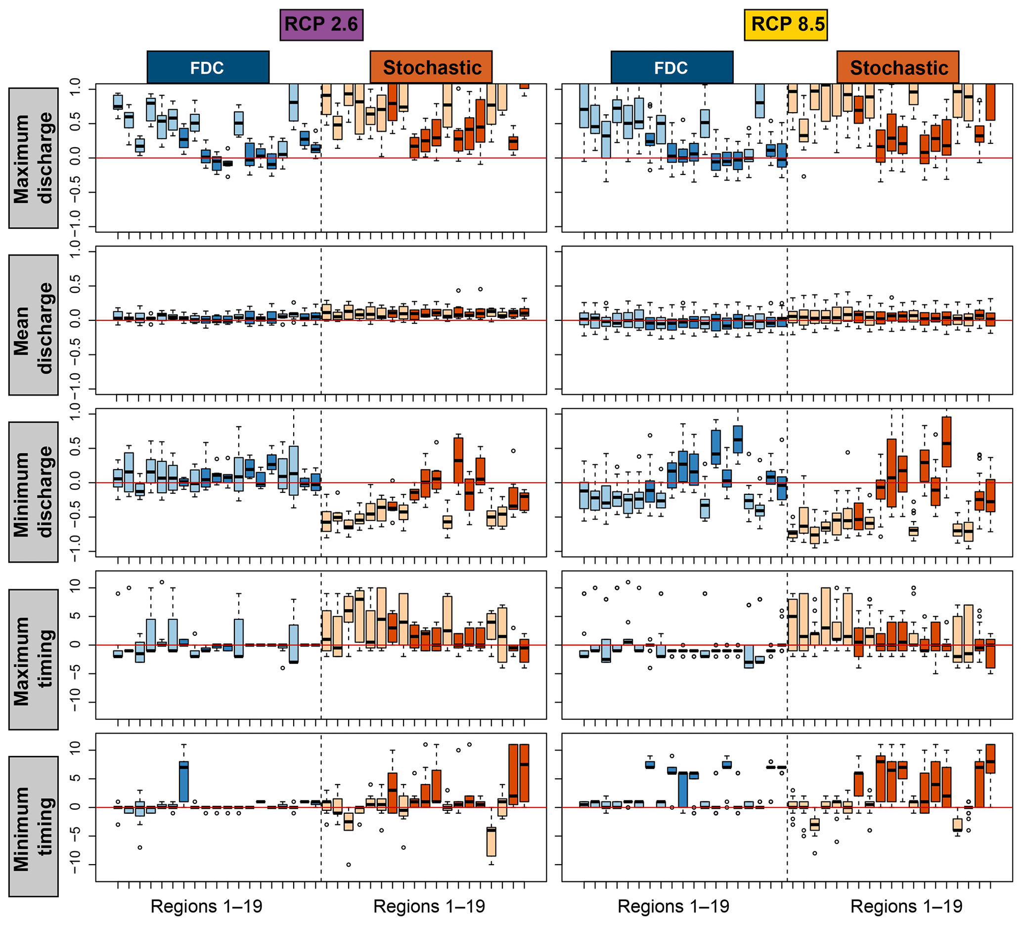
Figure 10Differences between current (i.e., multi-model mean of reference simulations) and future mean (grey) and extreme high-flow regime characteristics for the 19 regions (Fig. 1) estimated by the FDC (blue) and stochastic (orange) approaches. Five indicators are shown: maximum discharge, mean discharge, minimum discharge, timing of minimum discharge, and timing of maximum discharge. The first three rows show relative changes, the last two rows changes in months. Melt-dominated (dark colors) and rainfall-dominated (light colors) regions are distinguished. The boxplots indicate the range resulting from using the 39 GCM–RCM combinations for different scenarios.
4.1 Estimation methods
The low-flow regime estimates derived with the univariate method are implausible because the method neglects the interdependence between flows of adjacent months. In contrast, both other methods, FDC and stochastic, lead to similar results. The differences between the two methods mainly lie in how the seasonality is derived. In the case of the FDC approach, mean seasonality is used. In the case of the stochastic approach, a rather “random” seasonality is used since the regime is chosen according to the annual discharge sum. The use of one potential realization of seasonality in the stochastic approach compared to the use of a mean seasonality in the FDC approach has the disadvantage that it is less representative but the advantage that it is consistent with the corresponding annual discharge sum. The direction of changes derived from the two estimates are similar except for changes in minimum discharge in the low-flow regime and minimum discharge in the high-flow regimes. Both types of estimates seem to be plausible in the light of the stochastically generated hydrographs, which represent a large set of possible realizations among which extreme hydrographs can be found. While the estimates derived by the two methods do not differ much, both methods have their advantages and disadvantages. The FDC approach is relatively simple to implement but decouples seasonality from the distribution of daily discharge values. In contrast, the stochastic approach jointly considers magnitude and seasonality but requires the implementation of a stochastic discharge generator. The main advantage of such a generator is that the individual hydrograph realizations can be used for specific impact studies, which allows for direct performance of the frequency analysis of the quantity of interest. There are several possible solutions to the multivariate problem of estimating extreme regimes, and none of these two methods can therefore be said to be the better one.
The estimation of extremes, be it of regimes or individual flow characteristics, is associated with several sources of uncertainty. These comprise the choice of an extreme value distribution used to fit the data (i.e., percentiles of FDCs, annual sums, daily discharge sums) and the estimation of its parameters (Merz and Thieken, 2005; Brunner et al., 2018a). When applied to time series representing future conditions simulated with a hydrological model, additional uncertainty sources are involved. These include the assumptions underlying the applied future global climate scenarios, global climate model structures, initial conditions, downscaling methods, modeled future glacier extents, the uncertainties inherent in the hydrological model results, and the calibration of its parameters (Wilby et al., 2008; Addor et al., 2014; Clark et al., 2016). Despite these uncertainties, the extreme regime estimates can be used to identify future changes, and as such these estimates can be further used in climate impact studies. Potential fields of application include water scarcity assessments, where such regime estimates are combined with estimates of water demand (Brunner et al., 2018b), eco-hydrological studies (Wood et al., 2008), or analyses of the future potential of hydropower production (Schaefli et al., 2019).
4.2 Changes in future regime estimates
Changes in all types of regimes (mean/extreme low flow/extreme high flow) were found to be distinct for melt-dominated and rainfall-dominated regions. This refers not only to the entire regime, but also to individual regime characteristics such as minimum, maximum, and mean flow as well as the timing of the minimum flow. The direction of change was different in rainfall- and melt-dominated regions for all regime types. An increase of up to 50 % in the maximum discharge of mean and extreme low- and extreme high-flow regimes was found for rainfall-dominated regions. In contrast, a decrease in the minimum discharge by up to 100 % is projected to occur for these catchments and all types of regimes. The opposite is true for melt-dominated regimes, where the minimum discharge increases while the maximum and mean discharges decrease. The changes in extreme regimes can be explained by a reduction or an earlier contribution of snowmelt and glacier melt (Hanzer et al., 2018) and by an increase in winter precipitation (Jenicek et al., 2018), which coincide with the high-flow season in rainfall-dominated regions but with the low-flow season in melt-dominated regions. For mean regimes, changes in melt-dominated regimes were found in previous studies (Barnett et al., 2005; Jenicek et al., 2018; Fatichi et al., 2014; Hanzer et al., 2018). Fatichi et al. (2014) found a projected discharge decrease in melt-dominated regions due to reduced contribution of ice melt in the Po and Rhine river basins. The regime shifts in the rainfall-dominated regions are also influenced by increases in precipitation in the winter season and decreases in the summer season. Precipitation increases in the high-flow winter season lead to increases in the discharge maximum, while precipitation decreases in the low-flow summer season lead to decreases in the discharge minimum. The results of Fatichi et al. (2014) confirm that changes in rainfall-dominated regions are more uncertain since the projected changes in precipitation mostly lie within the range of natural variability of the control scenario. Similar results were found by Jenicek et al. (2018) for several catchments in Switzerland and by Barnett et al. (2005) on a global scale. We have shown here that these previous findings also apply to extreme regimes. The regime shifts detected have implications for various sectors. Regime shifts and more severe low flows were found to lead to more severe water scarcity situations, where water supply is insufficient to meet water demand (Brunner et al., 2019b). In the hydropower sector, future regime shifts are anticipated to lead to a reduction in production (Finger et al., 2012; Schaefli et al., 2019).
Extreme regime estimates were derived by frequency analysis performed on (1) annual flow duration curves (FDCs) and (2) the discharge sums of stochastically generated annual hydrographs. Both were found to provide realistic, similar results. A range of future extreme regime estimates was obtained for both extreme and mean conditions. In rainfall-dominated regions, the range of these future low- and high-flow estimates comprised the current estimate. In contrast, in melt-dominated regions, future high-flow and especially low-flow regimes were distinct from the current estimate. Changes in mean discharges were moderate for all types of regimes and catchments and did not exceed 30 %. Projected changes in the minimum discharge of mean and extreme high- and low-flow regimes were positive in melt-dominated regions due to increases in winter precipitation and amount to up to 100 %. In contrast, mostly positive changes of up to 50 % in maximum discharge were found in rainfall-dominated regions for all types of regimes. These positive changes in maximum discharge are linked to increases in winter precipitation, which coincide with the high-flow season. High- and low-flow regime estimates derived using the approaches proposed in this study are important for climate impact studies addressing, e.g., the future hydropower production potential or the occurrence of water shortage situations. The estimates also provide guidance for hydraulic design, emergency planning, and drought and water management.
The climate model simulations are available on the web page of the Swiss National Centre for Climate Services (https://www.nccs.admin.ch/nccs/de/home.html, NCCS, 2018). The hydrological model simulations are available upon request from Massimiliano Zappa (massimiliano.zappa@wsl.ch). The extreme regime estimates are available upon request from Manuela I. Brunner (manuela.brunner@wsl.ch).
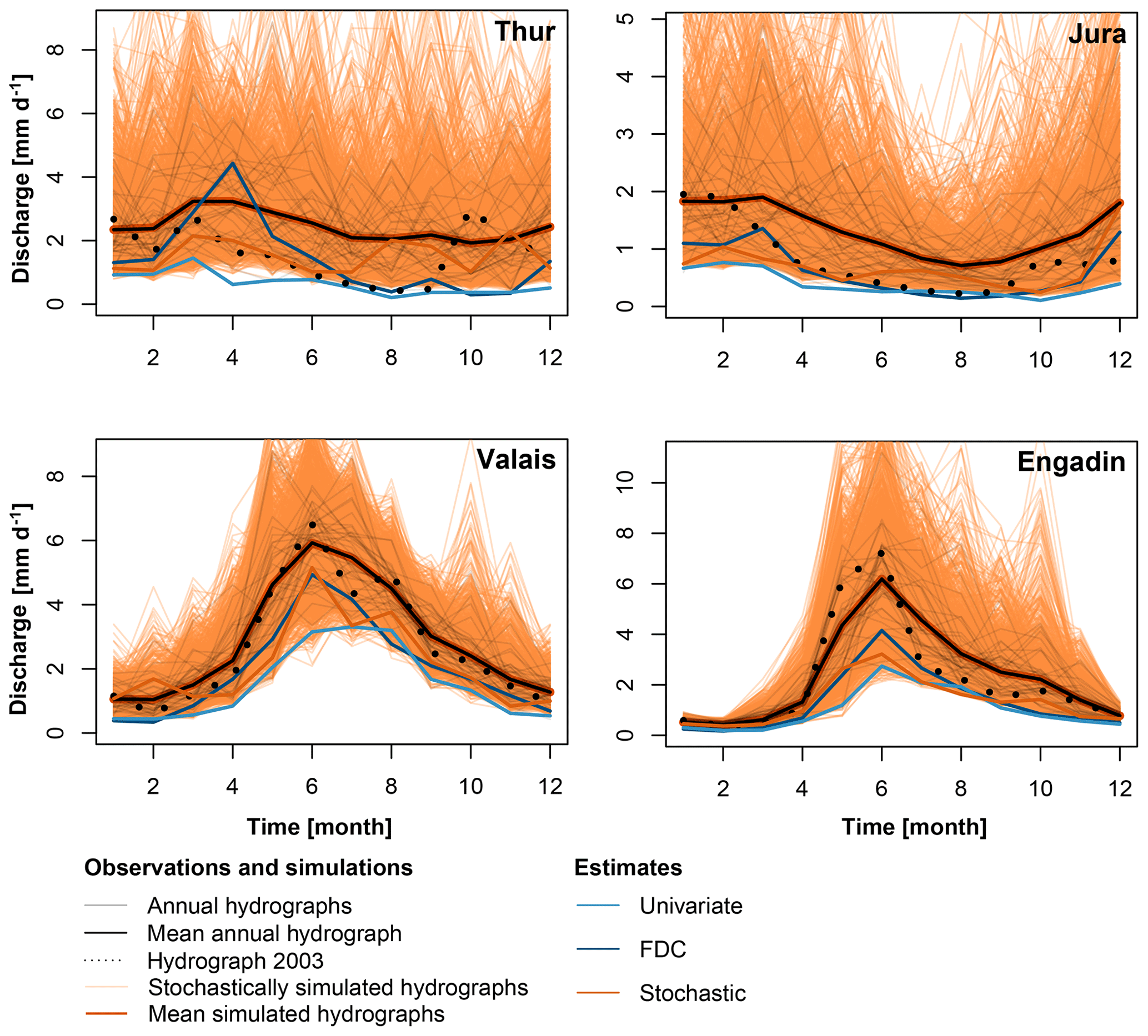
Figure A1Comparison of the 100-year low-flow regime estimates univariate, FDC, and stochastic with stochastically generated hydrographs (orange lines). The observed mean hydrograph (solid line) and the hydrograph of the year 2003 (dotted line) are given in black.
Table A1Summary of the 39 climate chains considered: global circulation model (GCM), regional climate model (RCM), representative concentration pathway (RCP), and grid cell resolution.
The idea and setup for the analyses were developed by MIB. MZ did the hydrological model simulations. HZ, MH, and DF provided the future glacier extents. The analyses were performed by MIB and discussed with MZ and DF. MIB wrote the first draft of the manuscript, which was revised by all the co-authors and edited by MIB.
The authors declare that they have no conflict of interest.
We thank MeteoSwiss for providing observed meteorological data and the Swiss National Centre for Climate Services (NCCS) for providing the climate model simulations.
This research has been supported by the Swiss Federal Office for the Environment (FOEN) (grant no. 15.0003.PJ/Q292-5096).
This paper was edited by Axel Bronstert and reviewed by two anonymous referees.
Addor, N., Rössler, O., Köplin, N., Huss, M., Weingartner, R., and Seibert, J.: Robust changes and sources of uncertainty in the projected hydrological regimes of Swiss catchments, Water Resour. Res., 50, 1–22, https://doi.org/10.1002/2014WR015549, 2014. a, b, c
Alderlieste, M., Van Lanen, H., and Wanders, N.: Future low flows and hydrological drought: How certain are these for Europe?, in: Proceedings of FRIEND-Water 2014, vol. 363, IAHS, Montpellier, 60–65, 2014. a
Anghileri, D., Voisin, N., Castelletti, A., Pianosi, F., Nijssen, B., and Lettenmaier, D.: Value of long-term streamflow forecasts to reservoir operations for water supply in snow-dominated river catchments, Water Resour. Res., 52, 4209–4225, https://doi.org/10.1002/2015WR017864, 2016. a
Aon Benfield: 2016 annual global climate and catastrophe report, Tech. rep., Aon Benfield, available at: http://thoughtleadership.aonbenfield.com/Documents/20170117-ab-if-annual-climate-catastrophe-report.pdf (last access: 15 March 2019), 2016. a
Arnell, N. W.: The effect of climate change on hydrological regimes in Europe, Global Environ. Change, 9, 5–23, https://doi.org/10.1016/S0959-3780(98)00015-6, 1999. a
Barnett, T. P., Adam, J. C., and Lettenmaier, D. P.: Potential impacts of a warming climate on water availability in snow-dominated regions, Nature, 438, 303–309, https://doi.org/10.1038/nature04141, 2005. a, b
Beniston, M.: The 2003 heat wave in Europe: A shape of things to come? An analysis based on Swiss climatological data and model simulations, Geophys. Res. Lett., 31, L02202, https://doi.org/10.1029/2003GL018857, 2004. a
Beniston, M., Farinotti, D., Stoffel, M., Andreassen, L. M., Coppola, E., Eckert, N., Fantini, A., Giacona, F., Hauck, C., Huss, M., Huwald, H., Lehning, M., López-Moreno, J. I., Magnusson, J., Marty, C., Morán-Tejéda, E., Morin, S., Naaim, M., Provenzale, A., Rabatel, A., Six, D., Stötter, J., Strasser, U., Terzago, S., and Vincent, C.: The European mountain cryosphere: A review of its current state, trends, and future challenges, The Cryosphere, 12, 759–794, https://doi.org/10.5194/tc-12-759-2018, 2018. a
Berghuijs, W. R., Woods, R. A., Hutton, C. J., and Sivapalan, M.: Dominant flood generating mechanisms across the United States, Geophys. Res. Lett., 43, 4382–4390, https://doi.org/10.1002/2016GL068070, 2016. a
Blöschl, G., Hall, J., Parajka, J., Perdigão, R. A. P., Merz, B., Arheimer, B., Aronica, G. T., Bilibashi, A., Bonacci, O., Borga, M., Ivan, C., Castellarin, A., and Chirico, G. B.: Changing climate shifts timing of European floods, Science, 357, 588–590, https://doi.org/10.1126/science.aan2506, 2017. a
Brönnimann, S., Rajczak, J., Fischer, E., Raible, C., Rohrer, M., and Schär, C.: Changing seasonality of moderate and extreme precipitation events in the Alps, Nat. Hazards Earth Syst. Sci., 18, 2047–2056, https://doi.org/10.5194/nhess-18-2047-2018, 2018. a
Brunner, M. I., Viviroli, D., Sikorska, A. E., Vannier, O., Favre, A.-C., and Seibert, J.: Flood type specific construction of synthetic design hydrographs, Water Resour. Res., 53, 1390–1406, https://doi.org/10.1002/2016WR019535, 2017. a
Brunner, M. I., Sikorska, A. E., Furrer, R., and Favre, A.-C.: Uncertainty assessment of synthetic design hydrographs for gauged and ungauged catchments, Water Resour. Res., 54, WR021129, https://doi.org/10.1002/2017WR021129, 2018a. a
Brunner, M. I., Zappa, M., and Stähli, M.: Scale matters: effects of temporal and spatial data resolution on water scarcity assessments, Adv. Water Resour., 123, 134–144, https://doi.org/10.1016/j.advwatres.2018.11.013, 2018b. a
Brunner, M. I., Bárdossy, A., and Furrer, R.: Technical note: Stochastic simulation of streamflow time series using phase randomization, Hydrol. Earth Syst. Sci., 23, 3175–3187, https://doi.org/10.5194/hess-23-3175-2019, 2019a. a, b, c
Brunner, M. I., Björnsen Gurung, A., Zappa, M., Zekollari, H., Farinotti, D., and Stähli, M.: Present and future water scarcity in Switzerland: Potential for alleviation through reservoirs and lakes, Sci. Total Environ., 666, 1033–1047, https://doi.org/10.1016/j.scitotenv.2019.02.169, 2019b. a, b
Castellarin, A., Vogel, R. M., and Brath, A.: A stochastic index flow model of flow duration curves, Water Resour. Res., 40, 1–10, https://doi.org/10.1029/2003WR002524, 2004. a
Chen, G. and Balakrishnan, N.: A general purpose approximate goodness-of-fit test, J. Qual. Technol., 2, 154–161, 1995. a
Claps, P. and Fiorentino, M.: Probabilistic flow duration curve for use in environmental planning and management, in: Integrated approach to environmental data management systems, edited by: Harmancioglu, N. B., Alpaslan, M. N., Ozkul, S. D., and Singh, V. P., Springer, Dordrecht, 255–266, 1997. a
Clark, M. P., Wilby, R. L., Gutmann, E. D., Vano, J. A., Gangopadhyay, S., Wood, A. W., Fowler, H. J., Prudhomme, C., Arnold, J. R., and Brekke, L. D.: Characterizing uncertainty of the hydrologic impacts of climate change, Curr. Clim. Change Rep., 2, 55–64, https://doi.org/10.1007/s40641-016-0034-x, 2016. a
Clarvis, M. H., Fatichi, S., Allan, A., Fuhrer, J., Stoffel, M., Romerio, F., Gaudard, L., Burlando, P., Beniston, M., Xoplaki, E., and Toreti, A.: Governing and managing water resources under changing hydro-climatic contexts: The case of the upper Rhone basin, Environ. Sci. Policy, 43, 56–67, https://doi.org/10.1016/j.envsci.2013.11.005, 2014. a
Farinotti, D., Pistocchi, A., and Huss, M.: From dwindling ice to headwater lakes: could dams replace glaciers in the European Alps?, Environ. Res. Lett., 11, 054022, https://doi.org/10.1088/1748-9326/11/5/054022, 2016. a
Fatichi, S., Rimkus, S., Burlando, P., and Bordoy, R.: Does internal climate variability overwhelm climate change signals in streamflow? The upper Po and Rhone basin case studies, Sci. Total Environ., 493, 1171–1182, https://doi.org/10.1016/j.scitotenv.2013.12.014, 2014. a, b, c
Federal Office of Meteorology and Climatology MeteoSwiss: Automatic monitoring network, available at: https://www.meteoswiss.admin.ch/home/measurement-and-forecasting-systems/land-based-stations/automatisches-messnetz.html, last access: 12 May 2018. a
Finger, D., Heinrich, G., Gobiet, A., and Bauder, A.: Projections of future water resources and their uncertainty in a glacierized catchment in the Swiss Alps and the subsequent effects on hydropower production during the 21st century, Water Resour. Res., 48, 1–20, https://doi.org/10.1029/2011WR010733, 2012. a
Fleming, S. W., Marsh Lavenue, A., Aly, A. H., and Adams, A.: Practical applications of spectral analysis of hydrologic time series, Hydrol. Process., 16, 565–574, https://doi.org/10.1002/hyp.523, 2002. a
Gudmundsson, L., Bremnes, J. B., Haugen, J. E., and Engen-Skaugen, T.: Technical Note: Downscaling RCM precipitation to the station scale using statistical transformations – A comparison of methods, Hydrol. Earth Syst. Sci., 16, 3383–3390, https://doi.org/10.5194/hess-16-3383-2012, 2012. a
Hänggi, P. and Weingartner, R.: Variations in discharge volumes for hydropower generation in Switzerland, Water Resour. Manage., 26, 1231–1252, https://doi.org/10.1007/s11269-011-9956-1, 2012. a
Hanzer, F., Förster, K., Nemec, J., and Strasser, U.: Projected cryospheric and hydrological impacts of 21st century climate change in the Ötztal Alps (Austria) simulated using a physically based approach, Hydrol. Earth Syst. Sci., 22, 1593–1614, https://doi.org/10.5194/hess-22-1593-2018, 2018. a, b
Herman, J. D., Reed, P. M., Zeff, H. B., Characklis, G. W., and Lamontagne, J.: Synthetic drought scenario generation to support bottom-up water supply vulnerability assessments, J. Water Resour. Pl. Manage., 142, 1–13, https://doi.org/10.1061/(ASCE)WR.1943-5452.0000701, 2016. a, b
Horton, P., Schaefli, B., Mezghani, A., Hingray, B., and Musy, A.: Assessment of climate-change impacts on alpine discharge regimes with climate model uncertainty, Hydrol. Process., 20, 2091–2109, https://doi.org/10.1002/hyp.6197, 2006. a, b
Hosking, J. R. M.: Modeling persistence in hydrological time series using fractional differencing, Water Resour. Res., 20, 1898–1908, https://doi.org/10.1029/WR020i012p01898, 1984. a
Hosking, J. R. M.: The four-parameter kappa distribution, IBM J. Res. Dev., 38, 251–258, 1994. a, b
Huss, M. and Hock, R.: A new model for global glacier change and sea-level rise, Front. Earth Sci., 3, 1–22, https://doi.org/10.3389/feart.2015.00054, 2015. a
Huss, M., Jouvet, G., Farinotti, D., and Bauder, A.: Future high-mountain hydrology: A new parameterization of glacier retreat, Hydrol. Earth Syst. Sci., 14, 815–829, https://doi.org/10.5194/hess-14-815-2010, 2010. a
Iacobellis, V.: Probabilistic model for the estimation of T year flow duration curves, Water Resour. Res., 44, 1–13, https://doi.org/10.1029/2006WR005400, 2008. a
Jacob, D., Petersen, J., Eggert, B., Alias, A., Christensen, O. B., Bouwer, L. M., Braun, A., Colette, A., Déqué, M., Georgievski, G., Georgopoulou, E., Gobiet, A., Menut, L., Nikulin, G., Haensler, A., Hempelmann, N., Jones, C., Keuler, K., Kovats, S., Kröner, N., Kotlarski, S., Kriegsmann, A., Martin, E., van Meijgaard, E., Moseley, C., Pfeifer, S., Preuschmann, S., Radermacher, C., Radtke, K., Rechid, D., Rounsevell, M., Samuelsson, P., Somot, S., Soussana, J.-F., Teichmann, C., Valentini, R., Vautard, R., Weber, B., and Yiou, P.: EURO-CORDEX: new high-resolution climate change projections for European impact research, Reg. Environ. Change, 14, 563–578, https://doi.org/10.1007/s10113-013-0499-2, 2014. a
Jenicek, M., Seibert, J., and Staudinger, M.: Modeling of future changes in seasonal snowpack and impacts on summer low flows in Alpine catchments, Water Resour. Res., 54, 538–556, https://doi.org/10.1002/2017WR021648, 2018. a, b, c, d
Jouvet, G., Huss, M., Funk, M., and Blatter, H.: Modelling the retreat of Grosser Aletschgletscher, Switzerland, in a changing climate, J. Glaciol., 57, 1033–1045, https://doi.org/10.3189/002214311798843359, 2011. a
Köplin, N., Viviroli, D., Schädler, B., and Weingartner, R.: How does climate change affect mesoscale catchments in Switzerland? – A framework for a comprehensive assessment, Adv. Geosci., 27, 111–119, https://doi.org/10.5194/adgeo-27-111-2010, 2010. a, b
Kotlarski, S., Keuler, K., Christensen, O. B., Colette, A., Déqué, M., Gobiet, A., Goergen, K., Jacob, D., Lüthi, D., Van Meijgaard, E., Nikulin, G., Schär, C., Teichmann, C., Vautard, R., Warrach-Sagi, K., and Wulfmeyer, V.: Regional climate modeling on European scales: A joint standard evaluation of the EURO-CORDEX RCM ensemble, Geosci. Model Dev., 7, 1297–1333, https://doi.org/10.5194/gmd-7-1297-2014, 2014. a
Koutsoyiannis, D.: A generalized mathematical framework for stochastic simulation and forecast of hydrologic time series, Water Resour. Res., 36, 1519–1533, 2000. a, b
Krysanova, V., Donnelly, C., Gelfan, A., Gerten, D., Arheimer, B., Hattermann, F., and Kundzewicz, Z. W.: How the performance of hydrological models relates to credibility of projections under climate change, Hydrolog. Sci. J., 63, 696–720, https://doi.org/10.1080/02626667.2018.1446214, 2018. a
Laghari, A. N., Vanham, D., and Rauch, W.: To what extent does climate change result in a shift in Alpine hydrology? A case study in the Austrian Alps, Hydrolog. Sci. J., 57, 103–117, https://doi.org/10.1080/02626667.2011.637040, 2012. a
Madsen, H., Lawrence, D., Lang, M., Martinkova, M., and Kjeldsen, T.: Review of trend analysis and climate change projections of extreme precipitation and floods in Europe, J. Hydrol., 519, 3634–3650, https://doi.org/10.1016/j.jhydrol.2014.11.003, 2014. a
Mandelbrot, B. B.: Une classe de processus stochastiques homothetiques a soi: Application a la loi climatologique de H. E. Hurst, Comptes rendus de l'Académie des sciences, 260, 3274–3276, 1965. a
Mandelbrot, B. B.: A fast fractional Gaussian noise generator, Water Resour. Res., 7, 543–553, 1971. a
Marx, A., Kumar, R., Thober, S., Rakovec, O., Wanders, N., Zink, M., Wood, E. F., Pan, M., Sheffield, J., and Samaniego, L.: Climate change alters low flows in Europe under global warming of 1.5, 2, and 3 ∘C, Hydrol. Earth Syst. Sci., 22, 1017–1032, https://doi.org/10.5194/hess-22-1017-2018, 2018. a
Mediero, L., Jiménez-Alvarez, A., and Garrote, L.: Design flood hydrographs from the relationship between flood peak and volume, Hydrol. Earth Syst. Sci., 14, 2495–2505, https://doi.org/10.5194/hess-14-2495-2010, 2010. a
Meinshausen, M., Smith, S. J., Calvin, K., Daniel, J. S., Kainuma, M. L., Lamarque, J., Matsumoto, K., Montzka, S. A., Raper, S. C., Riahi, K., Thomson, A., Velders, G. J., and van Vuuren, D. P.: The RCP greenhouse gas concentrations and their extensions from 1765 to 2300, Climatic Change, 109, 213–241, https://doi.org/10.1007/s10584-011-0156-z, 2011. a
Mejia, J. M., Rodriguez‐Iturbe, I., and Dawdy, D. R.: Streamflow simulation: 2. The broken line process as a potential model for hydrologic simulation, Water Resour. Rese., 8, 931–941, https://doi.org/10.1029/WR008i004p00931, 1972. a
Merz, B. and Thieken, A. H.: Separating natural and epistemic uncertainty in flood frequency analysis, J. Hydrol., 309, 114–132, https://doi.org/10.1016/j.jhydrol.2004.11.015, 2005. a
Meyer, J., Kohn, I., Stahl, K., Hakala, K., Seibert, J., and Cannon, A. J.: Effects of univariate and multivariate bias correction on hydrological impact projections in alpine catchments, Hydrol. Earth Syst. Sci., 23, 1339–1354, https://doi.org/10.5194/hess-23-1339-2019, 2019. a
Milano, M., Reynard, E., Köplin, N., and Weingartner, R.: Climatic and anthropogenic changes in Western Switzerland: Impacts on water stress, Sci. Total Environ., 536, 12–24, https://doi.org/10.1016/j.scitotenv.2015.07.049, 2015. a, b
Morrison, N.: Introduction to Fourier analysis, 3rd Edn., John Wiley & Sons, Inc, New York, 1994. a
Moss, R. H., Edmonds, J. A., Hibbard, K. A., Manning, M. R., Rose, S. K., van Vuuren, D. P., Carter, T. R., Emori, S., Kainuma, M., Kram, T., Meehl, G. A., Mitchell, J. F. B., Nakicenovic, N., Riahi, K., Smith, S. J., Stouffer, R. J., Thomson, A. M., Weyant, J. P., and Wilbanks, T. J.: The next generation of scenarios for climate change research and assessment, Nature, 463, 747–756, https://doi.org/10.1038/nature08823, 2010. a
Mussá, F. E., Zhou, Y., Maskey, S., Masih, I., and Uhlenbrook, S.: Groundwater as an emergency source for drought mitigation in the Crocodile River catchment, South Africa, Hydrol. Earth Syst. Sci., 19, 1093–1106, https://doi.org/10.5194/hess-19-1093-2015, 2015. a
National Centre for Climate Services: CH2018 – Climate Scenarios for Switzerland, Tech. rep., NCCS, Zurich, 2018. a
NCCS – National Center for Climate Services: Swiss Climate Change Scenarios, available at: https://www.nccs.admin.ch/nccs/en/home/climate-cha (last access: 7 October 2019), 2018. a
Nied, M., Schröter, K., Lüdtke, S., Nguyen, V. D., and Merz, B.: What are the hydro-meteorological controls on flood characteristics?, J. Hydrol., 545, 310–326, https://doi.org/10.1016/j.jhydrol.2016.12.003, 2017. a
Papadimitriou, L. V., Koutroulis, A. G., Grillakis, M. G., and Tsanis, I. K.: High-end climate change impact on European runoff and low flows – Exploring the effects of forcing biases, Hydrol. Earth Syst. Sci., 20, 1785–1808, https://doi.org/10.5194/hess-20-1785-2016, 2016. a
Pender, D., Patidar, S., Pender, G., and Haynes, H.: Stochastic simulation of daily streamflow sequences using a hidden Markov model, Hydrol. Res., 47, 75–88, https://doi.org/10.2166/nh.2015.114, 2015. a, b
Poff, N. L., Allan, J. D., Bain, M. B. M., Karr, J. J. R., Prestegaard, K. L. K., Richter, B. B. D., Sparks, R. E. R., and Stromberg, J. J. C.: The natural flow regime: A paradigm for river conservation and restoration, BioScience, 47, 769–784, https://doi.org/10.2307/1313099, 1997. a
Radziejewski, M., Bardossy, A., and Kundzewicz, Z.: Detection of change in river flow using phase randomization, Hydrolog. Sci. J., 45, 547–558, https://doi.org/10.1080/02626660009492356, 2000. a, b
Rebetez, M., Mayer, H., Dupont, O., Schindler, D., Gartner, K., Kropp, J. P., and Menzel, A.: Heat and drought 2003 in Europe: a climate synthesis, Ann. Forest Sci., 63, 569–577, https://doi.org/10.1051/forest:2006043, 2006. a
Rolls, R. J., Leigh, C., and Sheldon, F.: Mechanistic effects of low-flow hydrology on riverine ecosystems: ecological principles and consequences of alteration, Freshwater Sci., 31, 1163–1186, https://doi.org/10.1899/12-002.1, 2012. a
Salas, J. D. and Lee, T.: Nonparametric simulation of single-site seasonal streamflows, J. Hydrol. Eng., 15, 284–296, https://doi.org/10.1061/(ASCE)HE.1943-5584.0000189, 2010. a
Schaefli, B., Manso, P., Fischer, M., Huss, M., and Farinotti, D.: The role of glacier retreat for Swiss hydropower production, Renewable Energy, 132, 615–627, https://doi.org/10.1016/j.renene.2018.07.104, 2019. a, b
Schär, C., Vidale, P. L., Lüthi, D., Frei, C., Häberli, C., Liniger, M. A., and Appenzeller, C.: The role of increasing temperature variability in European summer, Nature, 427, 332–336, https://doi.org/10.1038/nature02230.1, 2004. a
Schreiber, T. and Schmitz, A.: Surrogate time series, Physica D, 142, 346–382, https://doi.org/10.1016/S0167-2789(00)00043-9, 2000. a
Şen, Z.: Climate change, droughts, and water resources, in: Applied Drought Modeling, Prediction, and Mitigation, chap. 6, 1st Edn., Elsevier Inc., Amsterdam, 321–391, https://doi.org/10.1016/B978-0-12-802176-7.00006-7, 2015. a
Sharma, A., Tarboton, D. G., and Lall, U.: Streamflow simulation: a nonparametric approach, Water Resour. Res., 33, 291–308, 1997. a
Shumway, R. H. and Stoffer, D. S.: Time series analysis and its applications. With R examples, 4th Edn., Springer International Publishing AG, Cham, https://doi.org/10.1007/978-1-4419-7865-3, 2017. a
Speich, M. J., Bernhard, L., Teuling, A. J., and Zappa, M.: Application of bivariate mapping for hydrological classification and analysis of temporal change and scale effects in Switzerland, J. Hydrol., 523, 804–821, https://doi.org/10.1016/j.jhydrol.2015.01.086, 2015. a
Tallaksen, L.: Streamflow drought frequency analysis, in: Drought and drought mitigation in Europe, edited by: Vogt, J. and Somma, F., Kluwer Academic Publishers, Dordrecht, 103–117, 2000. a
Ternynck, C., Ali, M., Alaya, B., Chebana, F., Dabo-Niang, S., and Ouarda, T. B. M. J.: Streamflow hydrograph classification using functional data analysis, Am. Meteorol. Soc., 17, 327–344, https://doi.org/10.1175/JHM-D-14-0200.1, 2016. a
Theiler, J., Eubank, S., Longtin, A., Galdrikian, B., and Farmer, J. D.: Testing for nonlinearity in time series: the method of surrogate data, Physica D, 58, 77–94, https://doi.org/10.1016/0167-2789(92)90102-S, 1992. a, b, c
Themeßl, M. J., Gobiet, A., and Heinrich, G.: Empirical-statistical downscaling and error correction of regional climate models and its impact on the climate change signal, Climatic Change, 112, 449–468, https://doi.org/10.1007/s10584-011-0224-4, 2012. a
Tsoukalas, I., Makropoulos, C., and Koutsoyiannis, D.: Simulation of stochastic processes exhibiting any-range dependence and arbitrary marginal distributions, Water Resour. Res., 54, 9484–9513, https://doi.org/10.1029/2017WR022462, 2018. a, b, c
Van Loon, A. F.: Hydrological drought explained, Wiley Interdisciplin. Rev.: Water, 2, 359–392, https://doi.org/10.1002/wat2.1085, 2015. a, b
van Vuuren, D. P., Edmonds, J., Kainuma, M., Riahi, K., Thomson, A., Hibbard, K., Hurtt, G. C., Kram, T., Krey, V., Lamarque, J. F., Masui, T., Meinshausen, M., Nakicenovic, N., Smith, S. J., and Rose, S. K.: The representative concentration pathways: An overview, Climatic Change, 109, 5–31, https://doi.org/10.1007/s10584-011-0148-z, 2011. a
Viviroli, D., Mittelbach, H., Gurtz, J., and Weingartner, R.: Continuous simulation for flood estimation in ungauged mesoscale catchments of Switzerland – Part II: Parameter regionalisation and flood estimation results, J. Hydrol., 377, 208–225, https://doi.org/10.1016/j.jhydrol.2009.08.022, 2009a. a
Viviroli, D., Zappa, M., Gurtz, J., and Weingartner, R.: An introduction to the hydrological modelling system PREVAH and its pre- and post-processing-tools, Environ. Model. Softw., 24, 1209–1222, https://doi.org/10.1016/j.envsoft.2009.04.001, 2009b. a, b, c
Vogel, R. M. and Fennessey, N. M.: Flow-duration curves. I: new interpretation and confidence intervals, J. Water Resour. Pl. Manage., 120, 485–504, 1994. a, b, c
Wilby, R., Beven, K., and Reynard, N.: Climate change and fluvial flood risk in the UK: more of the same?, Hydrol. Process., 22, 2511–2523, https://doi.org/10.1002/hyp.6847, 2008. a
WMO: Manual on Low-flow Estimation and Prediction, Tech. Rep. 1029, WMO-No. 1029, World Meteorological Organization (WMO), Geneva, 2008. a
Wood, P. J., Hannah, D. M., and Sadler, J. P.: Hydroecology and ecohydrology: past, present and future, 1st Edn., Wiley, Chichester, 2008. a
Zampieri, M., D'Andrea, F., Vautard, R., Clais, P., de Noblet-Ducoudré, N., and Yiou, P.: Hot European summers and the role of soil moisture in the propagation of Mediterranean drought, J. Climate, 22, 4747–4758, https://doi.org/10.1175/2009JCLI2568.1, 2009. a
Zappa, M. and Kan, C.: Extreme heat and runoff extremes in the Swiss Alps, Nat. Hazards Earth Syst. Sci., 7, 375–389, https://doi.org/10.5194/nhess-7-375-2007, 2007. a
Zekollari, H., Fürst, J. J., and Huybrechts, P.: Modelling the evolution of Vadret da Morteratsch, Switzerland, since the Little Ice Age and into the future, J. Glaciol., 60, 1208–1220, https://doi.org/10.3189/2014JoG14J053, 2014. a
Zekollari, H., Huss, M., and Farinotti, D.: Modelling the future evolution of glaciers in the European Alps under the EURO-CORDEX RCM ensemble, The Cryosphere, 13, 1125–1146, https://doi.org/10.5194/tc-13-1125-2019, 2019. a