the Creative Commons Attribution 4.0 License.
the Creative Commons Attribution 4.0 License.
 | 19 Nov 2019
Effect of disdrometer type on rain drop size distribution characterisation: a new dataset for south-eastern Australia
Jayaram Pudashine
Alain Protat
Remko Uijlenhoet
Valentijn R. N. Pauwels
Alan Seed
Jeffrey P. Walker
Knowledge of the full rainfall drop size distribution (DSD) is critical for characterising liquid water precipitation for applications such as rainfall retrievals using electromagnetic signals and atmospheric model parameterisation. Southern Hemisphere temperate latitudes have a lack of DSD observations and their integrated variables. Laser-based disdrometers rely on the attenuation of a beam by falling particles and are currently the most commonly used type of instrument to observe the DSD. However, there remain questions on the accuracy and variability in the DSDs measured by co-located instruments, whether identical models, different models or from different manufacturers. In this study, raw and processed DSD observations obtained from two of the most commonly deployed laser disdrometers, namely the Parsivel1 from OTT and the Laser Precipitation Monitor (LPM) from Thies Clima, are analysed and compared. Four co-located instruments of each type were deployed over 3 years from 2014 to 2017 in the proximity of Melbourne, a region prone to coastal rainfall in south-eastern Australia. This dataset includes a total of approximately 1.5 million recorded minutes, including over 40 000 min of quality rainfall data common to all instruments, equivalent to a cumulative amount of rainfall ranging from 1093 to 1244 mm (depending on the instrument records) for a total of 318 rainfall events. Most of the events lasted between 20 and 40 min for rainfall amounts of 0.12 to 26.0 mm. The co-located LPM sensors show very similar observations, while the co-located Parsivel1 systems show significantly different results. The LPM recorded 1 to 2 orders of magnitude more smaller droplets for drop diameters below 0.6 mm compared to the Parsivel1, with differences increasing at higher rainfall rates. The LPM integrated variables showed systematically lower values compared to the Parsivel1. Radar reflectivity–rainfall rate (ZH–R) relationships and resulting potential errors are also presented. Specific ZH–R relations for drizzle and convective rainfall are also derived based on DSD collected for each instrument type. Variability of the DSD as observed by co-located instruments of the same manufacturer had little impact on the estimated ZH–R relationships for stratiform rainfall, but differs when considering convective rainfall relations or ZH–R relations fitted to all available data. Conversely, disdrometer-derived ZH–R relations as compared to the Marshall–Palmer relation ZH=200R1.6 led to a bias in rainfall rates for reflectivities of 50 dBZ of up to 21.6 mm h−1. This study provides an open-source high-resolution dataset of co-located DSD to further explore sampling effects at the micro scale, along with rainfall microstructure.


Detailed knowledge of local rain microphysics is important for a range of applications: to better understand hydro-meteorological regimes and climate characteristics of a specific region, to study interactions between atmospheric and land surface processes, but also to determine characteristics of cloud and precipitation formation. Since the advent of weather radar and associated rainfall nowcasting applications, quantitative knowledge of the rain microstructure and knowledge of hydrometeor size distributions within precipitating clouds has become of great importance in order to relate backscattered radar signals to quantitative precipitation amounts (Marshall et al., 1955; Uijlenhoet, 2001). More broadly, the energy in the form of microwaves travelling through the atmosphere is susceptible to attenuation by vapour or liquid water. A quantitative knowledge of rain microphysics is thus critical for understanding and predicting how signal propagation is altered by precipitation. The data sources include weather radars, radiometers, and microwave communications at ground level, in particular commercial microwave links (CMLs). Relations between quantitative precipitation estimates (QPEs) and microwave signal (back)scattering, e.g. reflectivity and attenuation, highly depend on the rain microstructure, and an accurate QPE therefore requires detailed knowledge of the rain microstructure (Uijlenhoet, 2001; Krajewski and Smith, 2002; Uijlenhoet et al., 2003a, b; Uijlenhoet and Sempere Torres, 2006; Adirosi et al., 2018).
Rain microphysical properties are typically characterised by particle or drop size distribution (PSD or DSD) and/or particle size and velocity distribution (PSVD). These are not routinely measured in situ in the cloud or aloft, but at ground level, where long-term deployments of observational instruments are feasible. Historical observations have relied on manual sampling including stain and oil immersion techniques (Fuchs and Petrjanoff, 1937; Nawaby, 1970; Kathiravelu et al., 2016). Automatic disdrometers have since been designed to measure PSD and/or PSVD using either mechanical impact principles, where the falling drops hit a pressure sensor which converts this into an electrical current (Joss and Waldvogel, 1967), or the laser-extinction principle (Illingworth and Stevens, 1987), whereby the falling particles modify the laser beam between an emitter and receiver from which the PSVD is derived, and finally a video-based principle (Kruger and Krajewski, 2002; Schönhuber et al., 2008), where a combination of high-speed line-scan cameras records the PSVD.
Each method and corresponding hardware variety have their advantages and drawbacks, leading to different uncertainties and errors in the measured PSVD and PSD. Typically, video disdrometers (two-dimensional video disdrometers or 2DVD) were initially considered the most reliable to accurately measure PSVD (Thurai et al., 2017), particularly for particles larger than 0.3 mm. Recent work has re-visited this and now considers the 2DVD to significantly underestimate small particles in particular (Thurai and Bringi, 2018). Long-term deployments are often difficult and cost-prohibitive, and as a result these 2DVD instruments have typically been deployed for short-term research experiments. Thurai et al. (2017) presented data from a Meteorological Particle Spectrometer (MPS) (Baumgardner et al., 2002), arguing its higher sensitivity and better accuracy for diameters below 1.1 mm as compared to the 2DVD, while the 2DVD was proven to be accurate above 0.7 mm. The most commonly used disdrometer types at present are the laser-based disdrometers (Kathiravelu et al., 2016; Angulo-Martinez et al., 2018), with only a handful of manufacturers commercialising such instruments. The most commonly used disdrometers, with the highest citations in the scientific literature, are the particle size and velocity Parsivels of the first and second (released in 2011) generations by OTT Hydromet. Another widely used disdrometer, based on the exact same principle but with differences in the hardware design and internal processing, is the Laser Precipitation Monitor (LPM) by Thies Clima (de Moraes Frasson et al., 2011; Sarkar et al., 2015). These are predominantly used in research settings and sometimes in operations where the only sought-after information is a precise and accurate estimate of the rainfall amount (Merenti-Välimäki et al., 2001).
Since all PSVD observations using sensing techniques are subject to biases and errors, one of the most relevant approaches to accurately determine DSD is to use co-located instruments, preferably of different types and brands, to compare and evaluate the estimates from different instrumental sources. Such approaches have been used to evaluate DSD measured simultaneously by Parsivel1 only (Tapiador et al., 2010; Jaffrain and Berne, 2011; Jaffrain et al., 2011; Jaffrain and Berne, 2012a), Parsivel and 2DVD (Raupach and Berne, 2015), Meteorological Particle Spectrometer (or Sensor) and 2DVD (Thurai et al., 2017; Thurai and Bringi, 2018), Parsivel1 and LPM (Petan et al., 2010) and Parsivel2 and LPM (Angulo-Martinez et al., 2018). Work assessing the accuracy and biases of Parsivel has been widespread, while evaluation of the Thies LPM has received comparatively little attention (Brawn and Upton, 2008; Adirosi et al., 2018; Angulo-Martinez et al., 2018). Detection ranges vary slightly between Parsivel and LPM, with the LPM having a lower particle size detection threshold. Angulo-Martinez et al. (2018) filtered the raw matrices to a common detection range to allow direct comparison. Nevertheless, they found significant differences between the disdrometer models for both the PSVD and the integrated DSD moments.
In Australia, DSD observations have been conducted for the tropical region near Darwin during extensive campaigns over the past 20 years (Dolan et al., 2013; Thompson et al., 2018). Furthermore, extensive campaigns have been conducted to monitor PSVD (Maki et al., 2001; Penide et al., 2013; Thurai et al., 2010), and recent dedicated research vessel campaigns over multiple years have led to characterisation of the Australian sector of the Southern Ocean, which influences Australian weather and climate (between latitudes of 40 and 65∘ S; Mace and Protat, 2018a, b). PSVDs were measured using optical disdrometers specifically designed for harsh environments (Klepp et al., 2018). However, a knowledge gap remains for the temperate mid-latitudes of Australia, which also seems to be the case for all the Southern Hemisphere mid-latitudes. In Australia, more than 80 % of the population lives in the main metropolitan areas that are located along the south-eastern coastline (Sarkar et al., 2018). This region is therefore of particular interest for improved rainfall estimation using remote sensing techniques such as weather radar, CML or satellite, which all rely on accurate parameterisations of the DSD properties. The objectives of this study are therefore to (1) evaluate the differences between raw and processed PSVD, DSD and derived integrated variables from two laser disdrometer types: the OTT Parsivel1 and the Clima Thies LPM; (2) provide a comprehensive quantitative description of the DSD for the Melbourne region and climate; and (3) develop reflectivity–rainfall rate and attenuation–rainfall rate relationships for this region. To achieve this, four co-located laser-based disdrometers of two manufacturers (OTT and Thies) were deployed over a 3-year period in Melbourne, Australia.
2.1 Experimental site and regional setup
The observational site was located at the Australian Bureau of Meteorology experimental research and educational site at Broadmeadows (Fig. 1), a Metropolitan suburb located north of Melbourne, Australia (37∘41′27.4668′′ S, 144∘56′54.186′′ E). The site is situated approximately 15 km from the Port Phillip Bay shoreline and 85 km from the Bass Strait ocean shoreline. The Melbourne metropolitan area is classified as a marine western coast climate (Cfb, Köppen–Geiger classification). The average cumulative rainfall precipitation recorded at Melbourne Airport (weather station 086282 operated by the Bureau of Meteorology), located 9 km west of the experimental site, was 535 mm for the 1970–2018 period with a monthly maximum in November of 62 mm and a monthly minimum in July of 36 mm. However, there is relatively little variation in the monthly rainfall amounts throughout the year. Most of the precipitation in the south-eastern coastal climate of Australia originates from the Bass Strait and the Southern Ocean. This specific part of the coastal area is partly within the rain shadow of the Otway ranges to the south-east, which reduces total precipitation amounts when coastal systems originate from the Bass Strait or the Southern Ocean (Verdon-Kidd and Kiem, 2009).
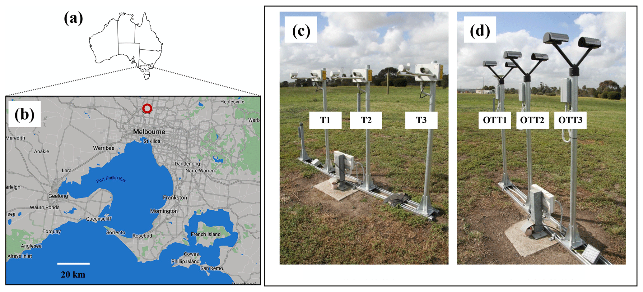
Figure 1(a, b) Location of the Melbourne metropolitan area within Australia (source: © Google Inc.) and the BoM experimental site at Broadmeadows (full circle); picture showing the disdrometers mounted on their stands at 1.5 m above the ground, (c) Thies Clima LPM (T1, T2, T3) and (d) OTT Parsivel1 (OTT1, OTT2, OTT3).
Six disdrometers were originally installed at the site (Fig. 1) in July 2014, three Thies Clima LPMs and three OTT Parsivel1, but only four instruments (two LPMs and two Parsivel1) operated continuously from July 2014 to July 2017. The other two instruments were relocated soon after the initial installation to other sites. All the instruments were installed on individual masts separated by 1.3 m and at a height of 1.5 m a.g.l. (above ground level) (Fig. 1). A distance of 2 m separated the Thies Clima LPM (T3) and the OTT Parsivel1 (OTT1) located on the edges of each of the rails (as seen in Fig. 1). The laser beams of the sensors were all oriented in the same direction (along the north–south axis) with raw 1 min data collected.
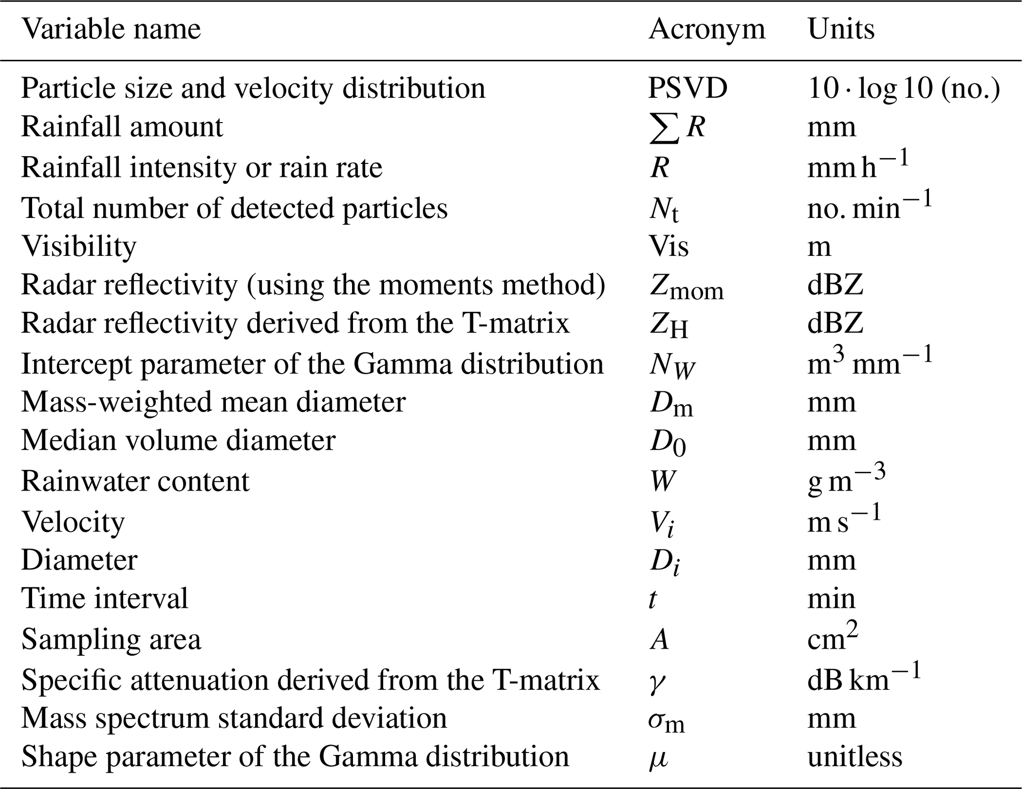
Both instrument types are based on a similar physical principle: the attenuation of the signal strength of an infrared laser when particles pass through the light beam. A common general principle for optical disdrometers is that their laser beam sheet has a negligible depth to sample the DSD. Both LPM and Parsivel1 consist of an emitter and a receiver (de Moraes Frasson et al., 2011) sampling an area of 45 to 55 cm2. In both cases, some processing is done within the internal parts of the units and the “raw” data are in fact already pre-processed, accounting for some corrections applied by the proprietary software. The “raw” data consist, for each sampling interval (in our case, 1 min), of a two-dimensional PSVD matrix where the first dimension is the diameter class and the second dimension is the velocity class. The number of particles falling into each combination of diameters and velocities is counted and recorded for each time interval. Integrated variables or “moments” are also computed from the PSVD matrix by the instruments' internal software and recorded for each time step, namely the rainfall amount (∑R, mm), rainfall intensity (R, mm h−1), horizontal radar reflectivity (ZH, dBZ), total number of detected particles (Nt, no. min−1) and visibility (Vis, m) (Table 1). In addition, synoptic weather codes defined by the World Meteorological Organization are also attributed to each 1 min DSD following software algorithms implemented by each manufacturer.
2.2 Parsivel1 from OTT
The Parsivel1 (Fig. 1) (OTT Hydromet Inc., USA) is made of two heads each mounted at the end of a V-shape, with the emitter and receiver being slightly protected at the source by a prominent splash protection shield. Parsivel1 uses a 650 nm laser beam generated by diodes covering an area of 54 cm2, corresponding to a distance between emitter and receiver of 180 mm and a beam width of 30 mm. The minimum sensitivity of the Parsivel1 corresponds to a particle size of 0.2 mm in diameter. The measured voltage drops when particles crossing the beam are converted into a 32 by 32 PSVD matrix with uneven bin sizes as described in Appendix A. The first two bin sizes for particle diameters (0–0.125 and 0.125–0.250) are systematically left empty. More details on the measurement procedure are described in Battaglia et al. (2010), Jaffrain et al. (2011), Tokay et al. (2013) and Angulo-Martinez et al. (2018). It is worth noting that a new version of the instrument was released by OTT in 2011 (Parsivel2), which incorporates some modifications from the version described herein (Tokay et al., 2014), including sensitivity to drop sizes in the lower and upper ranges. Specifically, Tokay et al. (2014) found the Parsivel2 to record more droplets in the three first measurable size bins as compared to Parsivel1 and fewer large drops as compared to Parsivel1. However, issues were identified on the recorded PSVD with underestimated velocities recorded by Parsivel2, while no issues were observed for Parsivel1.
2.3 Laser precipitation monitor from Thies Clima
The Laser Precipitation Monitor (LPM) (Fig. 1) (Thies Clima, Adolf Thies GmbH, Germany) is made of a central unit with the emitter diodes and a receiver forming an O-shape with brackets on each side of the beam. The Thies LPM uses a 785 nm laser beam covering an area of 45.6 cm2, corresponding to a distance between transmitter and receiver of 228 mm and a beam width of 20 mm. Similarly to the OTT Parsivel1, when a particle falls through the light beam, received signal strength is reduced and from that and the duration of the drop of signal level, particle number, sizes and their velocities are deduced for each time step using a proprietary software. The minimum sensitivity of the Thies LPM corresponds to a particle size of 0.16 mm in diameter. Measured voltage drops when particles cross the beam and are converted into a 22 by 20 PSVD matrix with uneven bin sizes as described in Appendix A. A number of quality flags are also provided for each time step to describe recorded PSVD and secondary derived data (or moments) quality.
2.4 Data processing
The 1 min time-step data were stored on a laptop located in a nearby building from the experimental site. Each of the instruments sent data “telegrams” after each completed min log, in the form of ASCII text data, which were then stored within the custom software on the PC. Generation of a new log file for each sensor occurred at midnight (local PC time). The PC was connected to the Internet, therefore allowing synchronisation of the internal clock. Synchronisation of the disdrometers was done every day using the PC to send “telegrams” to the units for time adjustments, in order to avoid time drifts. Data generated on a daily basis included raw PSVD matrices, additional derived moments and flags through various error codes.
Post-processing of the data was done using a pipeline written in the python language calling existing libraries such as pyDSD and pyTmatrix (see the section on software and model codes). First a series of filtering procedures was applied: (i) data corresponding to error flags were discarded; (ii) only data corresponding to WMO synoptic weather codes 4677 and 4680 for rainfall (drizzle, rain) were retained; (iii) following Jaffrain and Berne (2011), PSVD data needed to fall between ±50 % of the Atlas et al. (1973) drop velocity model to be retained. For the Thies LPM instruments, the upper bin classes for velocities (>10 m s−1) have no upper limit, but these data were retained; (iv) minute data must meet the occurrence of more than 10 particles in three different bins (Jaffrain and Berne, 2011; Tokay et al., 2013); (v) only rainfall rates > 0.1 mm h−1 were considered for further analysis; and (vi) contrary to Angulo-Martinez et al. (2018), the first bin diameter size for the LPM was used as, ultimately, users of this instrument will consider all available data to derive integrated DSD variables. The post-processed data following these sequential steps are further described as “quality” data. The sensitivity of the derived integrated variables to the smaller bin sizes was tested by computing DSD integrated variables considering either the full spectra or the DSD spectra for diameters > 0.6 mm. Table 2 summarises the statistics of the raw data and the data after applying the above successive filtering steps. Integrated variables provided by the instrument's internal software were only used for reference with integrated variables or moments computed from the filtered PSVD matrices. The drop size distributions were calculated using
where Di (mm) is the mean volume-equivalent diameter of the ith bin, N(Di) (m−3 mm−1) is the concentration of raindrops per unit volume in the interval from Di to Di+ΔDi, nij is the number of droplets recorded for measured fall speed Vj (m s−1) for velocity bin j, nd is the number of bins for velocities (32 for OTT and 20 for Thies), Ai (m2) is the effective sampling area for the ith size bin and Δt(s) is the sampling interval, equivalent to 60 s in this study. This effective sampling area Ai (m2) is calculated as per the equation below with ω (m2) the width of the laser beam.
Both the moments and T-matrix approaches were used to compute integrated variables to describe the microphysical properties of the sampled rainfall volumes, with the radar reflectivity factor Zmom (mm6 m−3) following
Rain rate R (mm h−1) was calculated as
with the generalised intercept parameter NW (m−3 mm−1) (or as defined by Testud et al., 2001) computed from
where ρw is the water density in g cm−3 and W is the rainwater content (g m−3) derived from
The largest value of the diameter for each DSD minute record is defined as Dmax (mm). The mass-weighted mean diameter Dm (mm) is finally calculated from
Surface horizontal reflectivity (ZH, dBZ) at the S-band was derived from the PSVD matrices using a python implementation (pyTmatrix) of the T-matrix approach (Leinonen, 2014). The default parameters including a canting angle of 12 ∘ (e.g. the standard deviation of a canting angle probability density function), the drop shape model of Brandes et al. (2002) and a temperature of 20 ∘C were used for the T-matrix calculations. ZH–R power relations were then calculated using an exponential power-law fit based upon a Levenberg–Marquardt minimisation (Moré, 1978). Sensitivity analysis of the T-matrix to the canting angle and temperature as well as a consistency analysis following a similar approach to Louf et al. (2019) were tested but not presented herein, as this is beyond the scope of the present study.
Table 2Summary of relevant statistics for the full dataset for the four co-located instruments.

Horizontal (γH, dB km−1) and vertical (γV, dB km−1) specific attenuations were also calculated using the same approach (Leinonen, 2014) using the same drop shape model and parameters. Both horizontal and vertical attenuations were calculated over the range of 0 to 70 GHz at intervals of 2 GHz. For each frequency, coefficients of the rainfall–attenuation (R=aγb) or attenuation–rainfall (γ=kRα) power relations were derived using an exponential power-law fit based upon a Levenberg–Marquardt minimisation (Moré, 1978). These were then compared with the International Telecommunication Union attenuation model for rainfall (ITU, 2005).
Each 1 min time step was classified as convective, stratiform or intermediate, following Islam et al. (2012). To examine the properties of the PSD for a range of rainfall regimes, each dataset was divided into five rain-rate classes: (a) 0.1–2 mm h−1; (b) 2–5 mm h−1; (c) 5–10 mm h−1; (d) 10–25 mm h−1; and (e) >25 mm h−1.
Observed DSDs were fitted using the Gamma distribution (Ulbrich, 1983):
where D (mm) is the particle diameter, N0 (m−3 mm) the intercept parameter, μ the shape parameter and Λ the slope parameter (mm−1). The method of Ulbrich and Atlas (1998) has been used to compute the intercept parameter, shape parameter and slope parameter using the method of moments. The list of parameters, units and abbreviations used in the equations is given in Table 1.
2.5 Auxiliary measurements
The closest tipping bucket rain gauge operating over that period was located at Essendon Airport (Bureau of Meteorology station no. 086038), being 5.6 km (37∘43′26.7708′′ S, 144∘54′21.7188′′ E) from the experimental site (Fig. 1). Another gauge located at Melbourne Airport (Bureau of Meteorology station no. 086282) and situated 9.0 km from the experimental site was also used for comparison. These data were used to compare with annual cumulative amounts, but given the distance have not been used for more quantitative analysis. Data from these two gauges were not filtered based on the disdrometer quality checks (given their distance from the experimental site) and therefore would likely record more total rainfall for the same period. Rainfall events were identified as meeting the criteria of no rainfall recorded for 30 min before the beginning and for 30 min after the end of the event.
3.1 Rainfall climatology for the 2014–2017 period
Table 2 presents relevant statistics that describe the full dataset obtained over 3 years for the four instruments. Approximately 1.5 million minutes of DSD were recorded by each of the instruments, the Thies LPM recording sensibly more minutes than the OTT Parsivel1 due to slight variations in the timing of installation and dismantling of the sensors. No error flags were observed for the OTT Parsivel1, while the Thies LPM recorded a number of erroneous data. The non-erroneous recorded combined rainfall, rainfall + drizzle and drizzle minutes, which were selected from the total minutes corresponding to liquid precipitation, accounting for approximately 6 % to 8 % of the total duration of the experiment (Table 2). A variety of precipitation types were observed at the site, including melting snow and hail, but these were anecdotal events covering hundreds of minutes only.
In this study, common minutes with rainfall rates above >0.1 mm h−1 measured by all four instruments were selected for analysis, following an approach similar to Angulo-Martinez et al. (2018). This corresponded to a total of 40 062 common quality (“quality” being defined as filtered and quality-checked data following the processing steps as described in the method section) minutes across the four instruments, with cumulative rainfall ranging from 1093 to 1244 mm (depending on the sensor) over the observational period. The two Thies LPM systems recorded very similar rainfall totals, while the two OTT Parsivel1 showed a difference of 89 mm between each Parsivel1 and above 100 mm when compared to the Thies LPM during the common observational period. Overall, the OTT Parsivel1 sensors always recorded more rainfall than the Thies LPM, despite their lower sensitivity (Fig. 2). The total amounts recorded by the operational tipping bucket rain gauges located 5.6 and 9.0 km from the disdrometers showed good agreement with the disdrometer records, with higher cumulative totals linked to the fact that these gauges were not filtered based on the disdrometer quality checks.
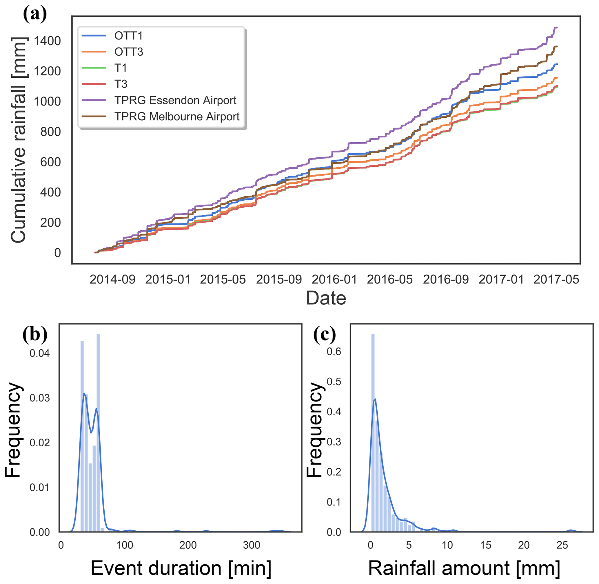
Figure 2(a) Cumulative rainfall amount for the July 2014 to July 2017 period for the four disdrometers and two tipping bucket rain gauges located at 5.6 km (Essendon Airport) and 9.0 km (Melbourne Airport); (b) rainfall event duration frequency distribution based on rainfall records from OTT1; (c) rainfall cumulative amounts per event frequency distribution based on rainfall records from OTT1.
Figure 2 also shows the frequency distribution of the 318 rainfall events, which follow an exponential distribution with the majority of events lasting between 20 and 40 min; the exception is 4 events lasting far longer, with the longest covering 340 min. The total rainfall amounts recorded per event varied from 0.12 to 26.0 mm (with instrument OTT3 taken as the reference here). Over these 3 years, rainfall was frequent all year long, with more occurrences in the Southern Hemisphere autumn and winter, and summer accounting for the lowest rainfall occurrence. The mean average annual rainfall over these 3 years is within the mean envelope of rainfall records observed for this region over the last century.
3.2 DSD for the full dataset
After a succession of quality checks and filtering as described in the previous section, the total number of observed particles for each of the instruments was derived per bin size. In order to directly compare the Thies LPM and OTT Parsivel1, which have differences in resolution and measurement sensitivity (Table A1), common bin ranges were used and the results plotted in Fig. 3. The Thies LPM instrument can measure smaller diameter drops as it includes a 0.125 to 0.25 mm bin size that the OTT Parsivel1 does not cover. Therefore only Thies LPM observations are plotted for that diameter range. From the 0.25 to 0.5 mm range, the Thies LPM instruments measured a considerably larger number of droplets than OTT Parsivel1, a feature documented in the literature (Chen et al., 2016; Angulo-Martinez et al., 2018), illustrating the higher sensitivity of the Thies LPM over the OTT Parsivel1. For the 0.5 to 0.75 mm range as well as the 1.5 to 3.0 mm range, a very consistent total number of droplets was measured across all instruments of both manufacturers. OTT Parsivel1 measured more droplets than the Thies LPM for the 0.75 to 1.5 mm range, which likely explains the higher total amount of rainfall measured over the 3 years by both OTT Parsivel1. For larger drop diameter ranges (>3 mm), the Thies LPM systematically recorded more droplets than the OTT Parsivel1, but their total numbers as compared to the middle-range diameter bins were orders of magnitude less. Very small differences can be observed between instruments of the same manufacturer (e.g. T1 versus T3 or OTT1 versus OTT3), with the larger discrepancies being observed at each end of the spectrum, e.g. for the lowest diameter bin for the Thies LPM, and the upper range of diameters for both OTT Parsivel1 and the Thies LPM. The observed differences for the lowest diameter bins are likely due to sensitivity differences between the Thies LPM instruments, while the differences for the largest diameter particle class range (6 to 7 mm) seen across all four instruments are likely due to sampling effects. The observed particles for the range 6 to 7 mm correspond only to between 3 and 8 recorded minutes (out of 40 062), depending on the instrument.
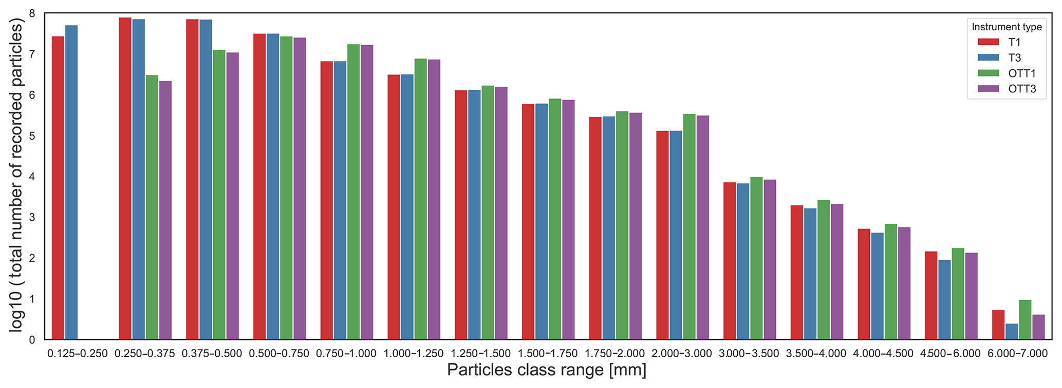
Figure 3Distribution of the recorded total number of particles per bin for each of the four co-located instruments.
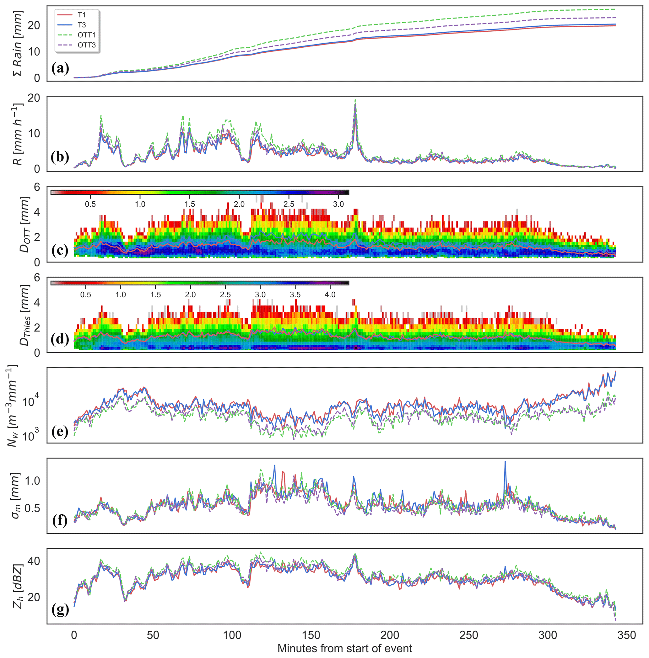
Figure 4Rainfall event no. 7 time series (the event started on 24 September 2014 at 09:09 AEDT) of (a) cumulative rainfall amounts (mm); (b) rainfall rate (mm h−1); (c) density distribution (log scale) of drop size diameters for OTT1 (mm); blue line is OTT1 Dm (mm) and red line is OTT3 Dm (mm); (d) density distribution (log scale) of drop size diameters for T1 (mm); blue line is OTT1 Dm (mm) and red line is OTT3 Dm (mm); (e) generalised intercept parameter (m−3 mm−1); (f) mass spectrum standard deviation (mm); and (g) horizontal reflectivity (dBZ).
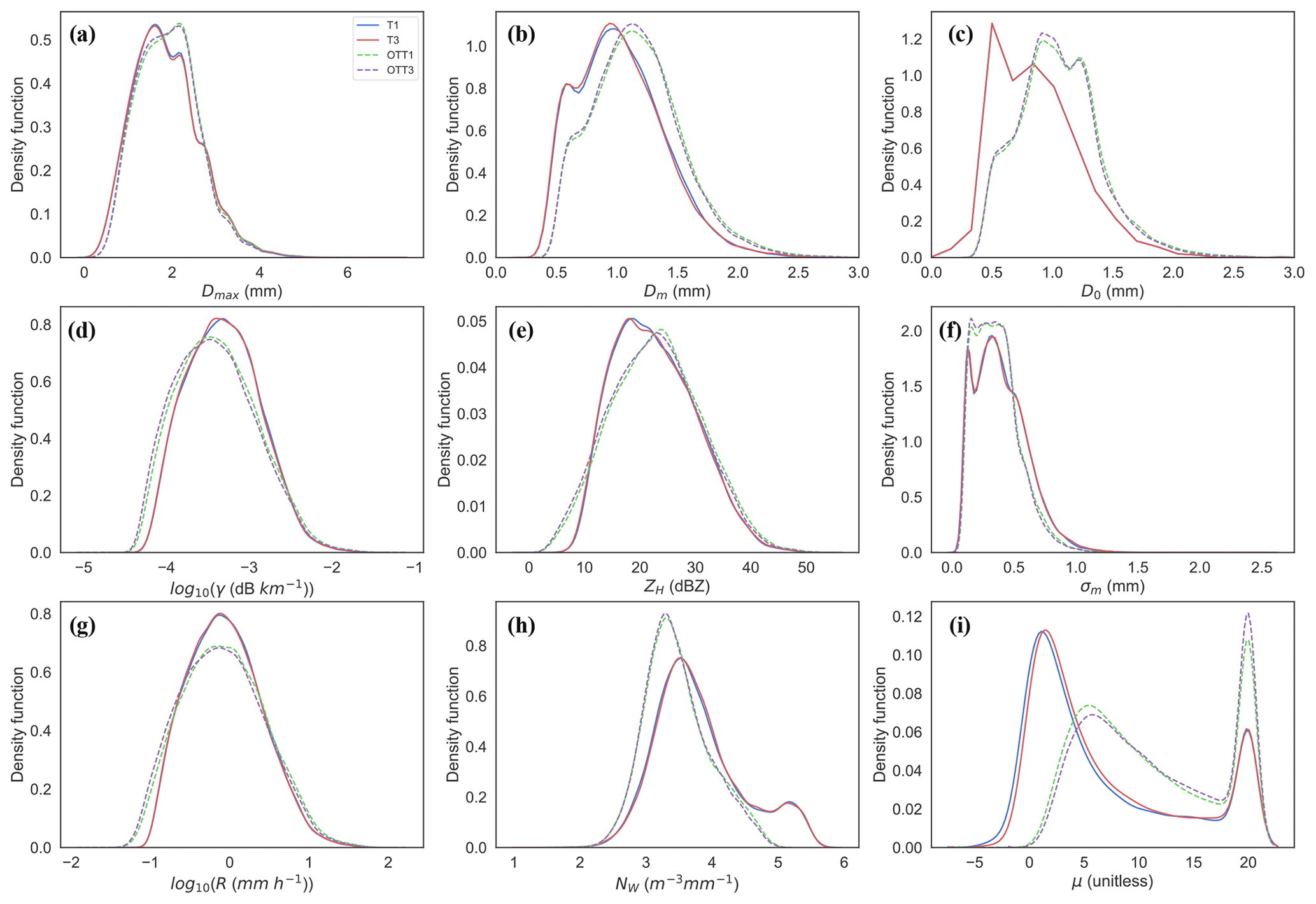
Figure 5Density estimates of the DSD parameters (Dmax, Dm, D0, γH, ZH, σm, R, NW and μ) for the four instruments (T1, T3, OTT1, OTT3) for the full dataset.
3.3 Detailed inter-comparison for a single event
The longest-duration event in the data was event no. 7, which lasted for 344 min and produced more than 20 mm of rain. Figure 4 shows the time series of integrated DSD variables (or moments) as well as the DSD spectrum as density plots. To facilitate readability, the full DSD graphs in Fig. 4c and d only show OTT1 and T1, as the instruments show very similar DSD characteristics across the event. For this event, the Thies LPM instruments presented a similar total rainfall amount ( and mm for T1 and T3, respectively), lower than OTT1 and OTT3 ( mm and mm, respectively). Differences were small between instruments for low rainfall rates, but large discrepancies are found for higher rainfall rates. OTT1 and OTT3 showed systematically higher rain rates than the Thies LPM, corresponding to more particles of large diameter recorded in the bins > 4 mm. There was also a larger number of droplets in the mid-range diameters. Conversely, the Thies LPM recorded more particles in total, as shown by the higher NW across the full event, with the largest differences for OTT Parsivel1 at low rainfall rates. While these differences in the total number of recorded particles are significant, they did not impact the horizontal reflectivity, which is sensitive to the number of large drops because ZH is equivalent to the sixth moment of the DSD. The OTT Parsivel1 instruments still showed a slightly higher reflectivity for the second part of high rain rates for this event (minutes 220 to 280).
3.4 Minute-resolution DSD
The kernel density estimation (KDE) technique (Sheather and Jones, 1991) was used to estimate the probability distribution of the observed DSD parameters for each of the 40 062 min that had good quality data for all four instruments. The frequency distributions of these parameters are shown in Fig. 5.
The frequency distribution of the parameters exhibits very little differences from the same manufacturer (OTT or Thies), but large differences were found between the Thies LPM and OTT Parsivel1 for the lower-order moments such as Dm, D0, σm, and Nw. A remarkable feature is the difference in the frequency distributions for Dm, D0 and σm due to the larger number of smaller droplets that were measured by the Thies LPM as compared to the OTT Parsivel1. These large numbers of particles recorded by the Thies LPM are identified in Nw as the peak towards larger values, which is not found in the OTT Parsivel1 statistics. The impact of this higher frequency of small droplets is a shift towards a smaller median reflectivity for the Thies LPM, while attenuation is on average higher for the Thies disdrometers as compared to the OTT Parsivel1. The shape of the Gamma distribution μ utilised to parameterise the DSD is substantially different between OTT Parsivel1 and the Thies LPM due to this larger number of smaller droplets for the Thies LPM. The μ distribution has a bimodal distribution with a first peak of 6.0 (OTT) or 0.0 (Thies) and a second peak at around 20.0 for both. This smaller value of μ0 for the Thies LPM corresponds to a different shape of the DSD influenced by a larger number of small diameters.
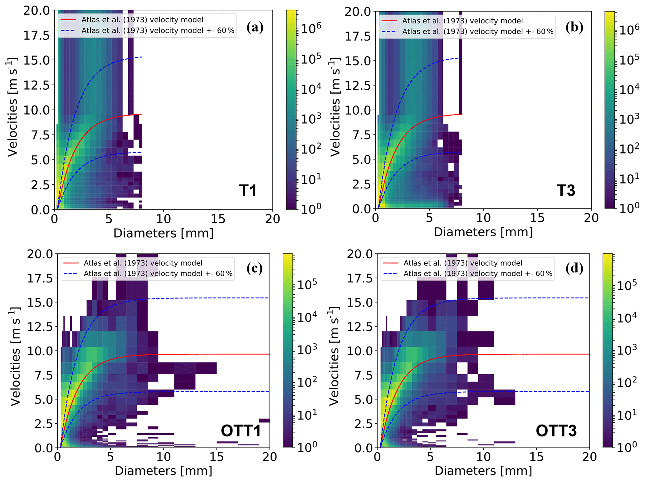
Figure 6Particle velocity versus diameter density plots for the 2014–2017 period for the four instruments. The colour scale indicates the number of particles for each bin (velocity and diameter). The velocity model of Atlas et al. (1973) is plotted in red together with its positive and negative deviations of 60 %. This is used to filter outliers following Jaffrain and Berne (2011).
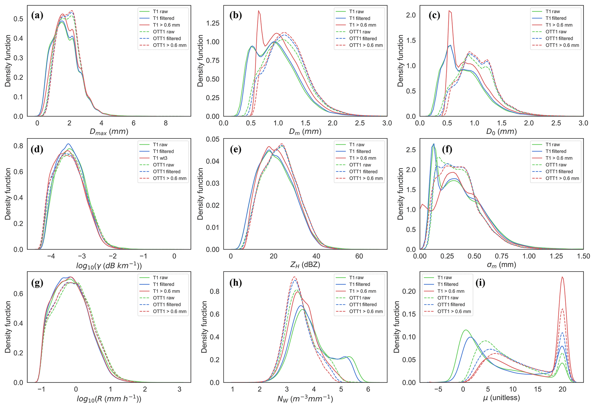
Figure 7Frequency plots of the DSD parameters, based on distributions (not shown) of integrated variables (Dmax, Dm, D0, γH, ZH, σm, R, NW and μ) for two instruments (OTT1 and T1) for the full dataset for rainfall rates > 0.1 mm h−1 and for raw data (green), filtered data (blue) and minute data meeting Dm>0.6 mm (red).
3.5 Effect of filtering and data correction on DSD parameters
The effect of some of the filtering and the presence of smaller droplets on the DSD parameters is analysed here through the means of the analysis shown in Figs. 6 and 7. Figure 6 shows the PSVD matrix density plots for the full period of observation for the four instruments as well as the boundaries used to eliminate the erroneous data as proposed by Jaffrain and Berne (2011), but using here the model of Atlas et al. (1973) instead of Beard (1977). The OTT Parsivel1 sampled a larger range of diameters and velocities as a result of their resolution and bin arrangement shown in Table A1. Relatively few droplets fell into the zones of low velocity/large diameters or high velocity/small diameters, while one of the Thies LPM instruments (T3) measured a very large number of particles falling into these two categories. This was hypothesised to be due to the design of the Thies LPM, increasing the probability to record more edge events (smaller sampling area) and the brackets surrounding the laser beam increasing the possibility of splashes, both contributing to a higher number of falsely identified rain droplets (Angulo-Martinez et al., 2018).
The effects of the filtering process on the frequency distribution of the DSD parameters can be seen in Fig. 7. Only one instrument of each manufacturer is shown for readability. The impact of the filtering was different for the two types of instruments. Only the fitting parameters Nw and μ0 as well as Dm were slightly affected for the Thies LPM. In contrast, the OTT Parsivel1 data were less affected, as expected since the OTT Parsivel1 recorded smaller number of droplets with diameter ranges < 0.6 mm.
One can also quantify the contribution of small diameter ranges (<0.6 mm) to the integrated variables through Fig. 7. For the Thies LPM, Dm and D0 showed a peak in the frequency distributions for the lower diameters above 0.6 mm after removing the smaller bin size records, as expected. This is because their relative contribution increased when removing highly frequent smaller bin ranges. This feature was not observed for the OTT Parsivel1, showing that the small diameter records were not much more frequent relative to the total number of recorded particles. Also as expected, the proportion of smaller rainfall rates was reduced for the Thies LPM when removing the smaller diameter bin sizes, since this instrument is highly sensitive to smaller droplets that contribute to both small and high rain rates. DSD moments of higher order showed less modification of their values when not considering diameter bins < 0.6 mm, since the smaller diameters contribute relatively less when the moment order increases (order 6 for ZH).
3.6 Properties of minute DSD variables for different rainfall rates
In order to explore the effect of the rainfall rate, KDEs of the integrated variables from minute DSD data for the four co-located instruments are shown in Appendix A (Figs. A1–A4) and in Fig. 8 for rainfall rates of 0.1–2, 2–5, 5–10, 10–25 and >25 mm h−1, respectively. Figure 8 shows the most pronounced differences corresponding to the highest rain rates. Differences between instruments of the same manufacturer increased with rain rate, in particular for OTT Parsivel1. OTT1 showed similar frequencies to OTT3 for rain rates, reflectivity and attenuation values, but in OTT1 there were more low values and less frequent mid-range values than in OTT3 distributions. Both Thies LPM statistics were similar. All DSD parameters (Fig. 8) started to show discrepancies between all instruments for rain rates > 10 mm h−1, due to the sampling effect related to the occurrence of larger drops falling erratically in space and time, therefore being captured by some instruments but not by co-located neighbours, this being enhanced by the small data sample (128 min of data in Fig. 8). Smaller values of μ0 for the Thies LPM indicate the presence of a larger number of small droplets (also seen in NW), therefore modifying the shape of the DSD towards the smaller normalised diameters.
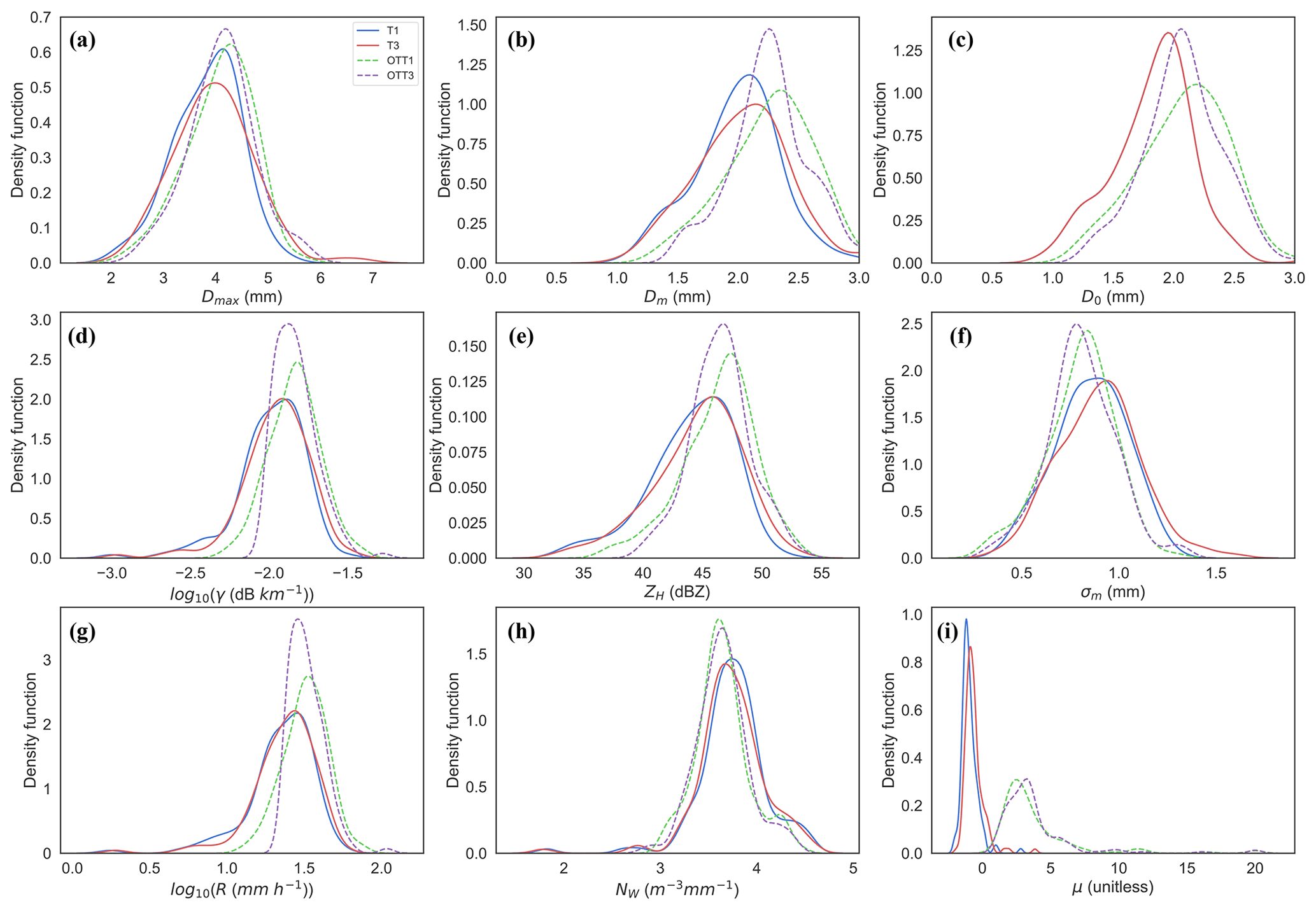
Figure 8Frequency plots of the DSD parameters, based on distributions (not shown) of integrated variables (Dmax, Dm, D0, γH, ZH, σm, R, NW and μ) for the four instruments (T1, T3, OTT1, OTT3) for R>25 mm h−1 (129 data points).
3.7 ZH–R and k–R relations
Horizontal reflectivity versus rainfall rate typically follows a simple power law such as ZH=aRb, as initially described by Marshall and Palmer (1948), with the coefficients of that power-law relation depending on the DSD properties (Uijlenhoet, 2001). Hence, it is of interest here to characterise the variability of such relationships among the four co-located instruments. Figure 9 shows the scatter plots together with fitted ZH–R relations, with the fitting being done for DSD corresponding to Dm<0.6 mm and to Dm>0.6 mm. Indeed, in the frequency distributions seen in the previous sections, integrated parameters of the DSD showed the occurrence of bimodal distributions (for NW, D0 and Dm in particular). That implies that when considering the full dataset, there should be at least two corresponding power-law relations for each distribution of the data. Distinct ZH–R relations for stratiform rainfall (Dm>0.6 mm) (with stratiform and convective simply differentiated here by a threshold value of >30 dBZ for convective), drizzle (Dm<0.6 mm) and convective rainfall (for ZH>30 dBZ) are shown in Table 3. Relationships considering all data are the closest to the Marshall–Palmer relations and differ significantly for stratiform rainfall for both instrument types.
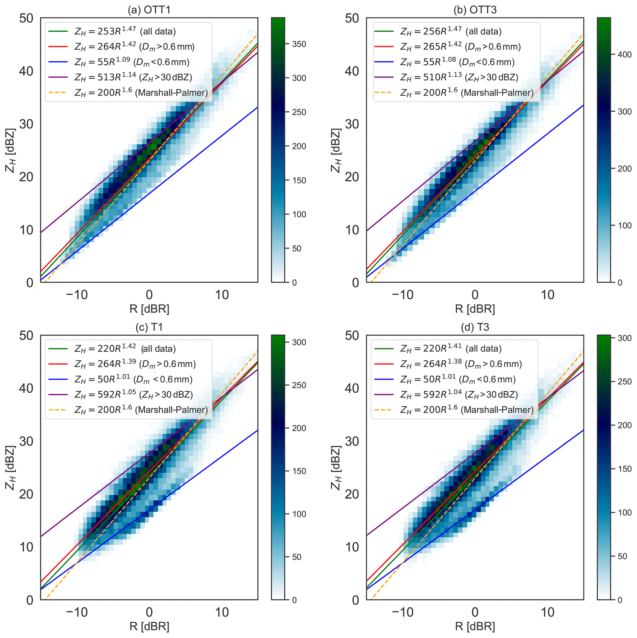
Figure 9Horizontal reflectivity (in 10log 10(ZH) – dBZ) versus rain rate (in 10log 10(R) – dBR) scatter plots for all co-located instruments (a–d). Power-law relations are fitted separately for all data, data meeting Dm>0.6 mm (red curves), data meeting Dm<0.6 mm (blue curves), and data meeting ZH>30 dBZ (purple curves). The reference Marshall–Palmer relation ZH=200R1.6 (Marshall et al., 1955) is also shown.
Table 3ZH–R relations for each of the co-located instruments corresponding to data fits to different subsets of data.
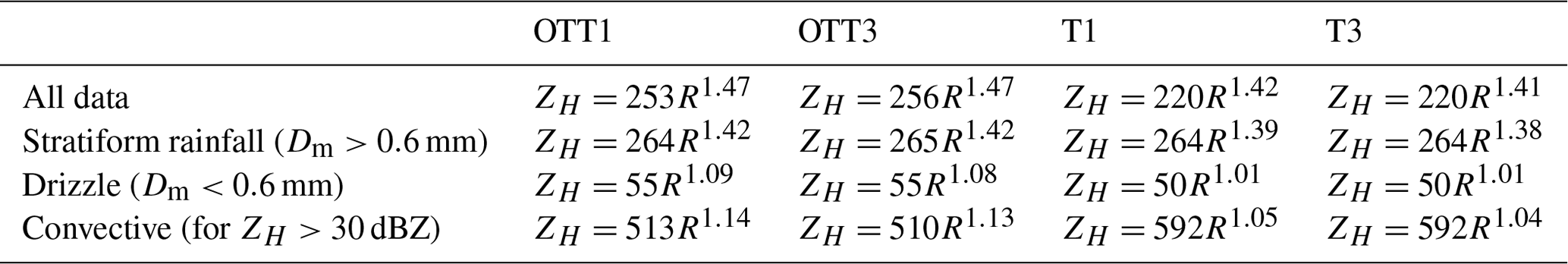
The power-law relations and related a and b coefficients were found to be very similar for the same instrument type (OTT Parsivel1 or the Thies LPM), but differed significantly between manufacturers when considering the full dataset for fitting the relations, and for convective rainfall. For stratiform rainfall (Dm>0.6 mm) coefficients were almost identical for the four instruments, which was expected given the similarity in the observations of the DSD across all instruments for the middle range of diameter bins.
ZH–R relations being directly related to the DSD, so are the coefficients a and b. Empirical observations and further demonstrations (Uijlenhoet, 2001; Uijlenhoet and Stricker, 1999; Uijlenhoet et al., 2003a) have shown that the value of coefficient a will tend to increase and the value of coefficient b to decrease as the raindrop mean diameter size increases and the concentration in the volume decreases, e.g. in the case of convective rainfall, in particular for thunderstorms. This is indeed what is observed here when comparing the relations for stratiform rainfall to the relations derived for convective rainfall and in the range of values observed in the literature to date (Uijlenhoet et al., 2003b, 2006).
The ZH–R relations for Dm<0.6 mm correspond to drizzle, which consists of essentially small drops. The existing literature on ZH–R relations for drizzle is confined to a few articles, with most of the observations having been made using aircraft-based instruments at cloud level. Comstock et al. (2004) report historical ZH–R relations for drizzle with varying a and b coefficients: ZH=150R1.5 (Joss and Waldvogel, 1969) and ZH=10R1.0 (Vali et al., 1998), with the Joss and Waldvogel (1969) b coefficient being estimated and not measured. Comstock et al. (2004) also reported their own measurements of ZH=25R1.3, ZH=32R1.4 and ZH=57R1.1. The estimates in Table 3 are within the range of those observations for drizzle, with a b coefficient closer to unity (indicating the so-called equilibrium precipitation, Uijlenhoet et al., 2003b), while there was a reduced value of the a coefficient as compared to rainfall. The vertical profile of DSDs above ground, in particular for stratiform clouds, is an entire field of research, and further discussion and analysis on that aspect should be conducted in a dedicated study. The findings of this paper showed that the Thies LPM has the capacity to capture this part of the DSD spectrum, although some additional research using co-located disdrometers also capturing this lower part of the DSD spectrum will be needed to evaluate the accuracy of these Thies LPM measurements.
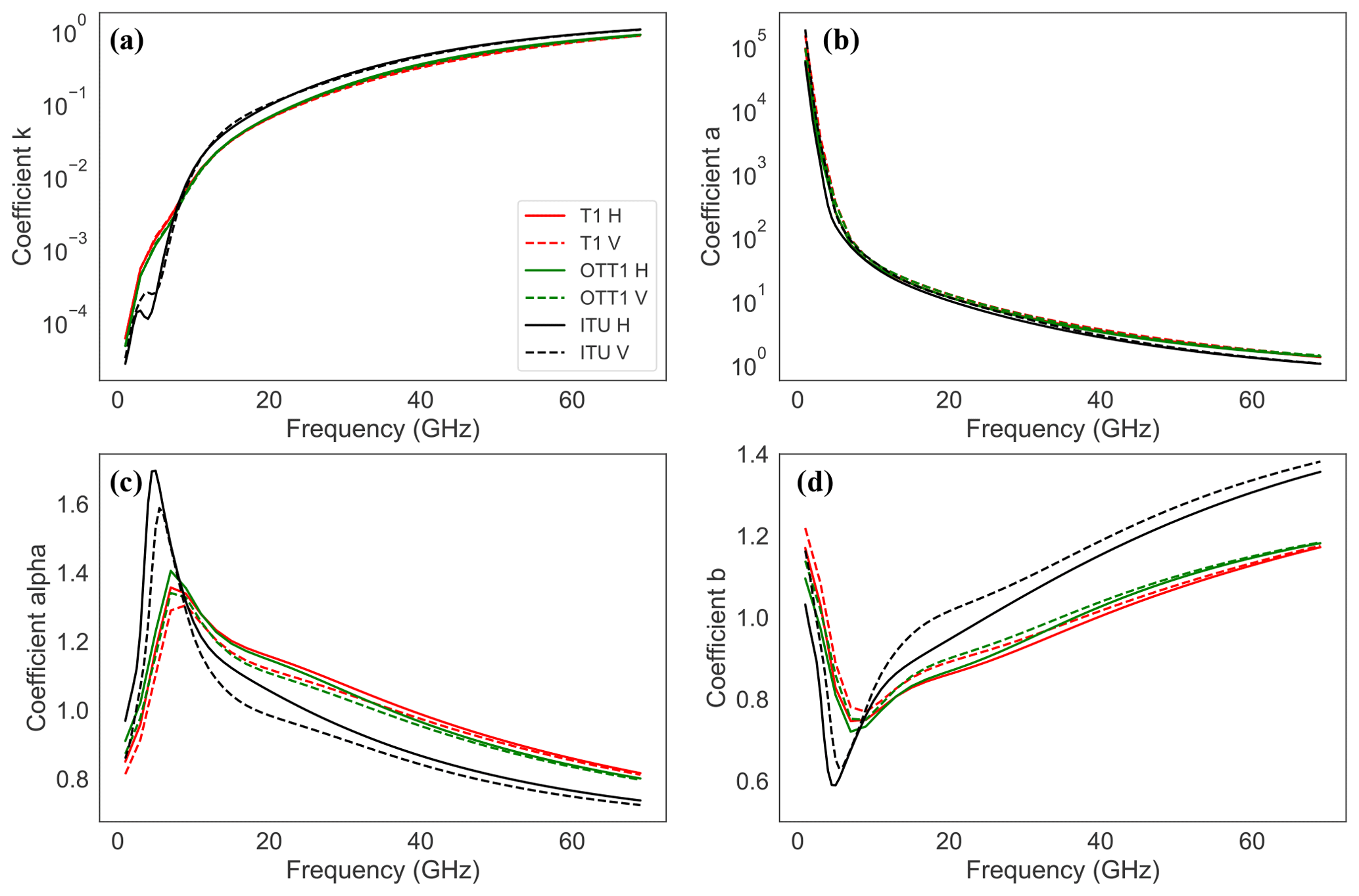
Figure 10Coefficients of the γ–R or R–γ relations for both horizontal and vertical polarisations derived from the full DSD dataset for Thies LPM T1 and OTT Parsivel1 OTT1. The black line represents the International Telecommunications Union model (ITU, 2005).
Table 4Differences in rainfall estimation following diverse fitted ZH–R relations based on each type (OTT or Thies) of instrument. T1 was taken as the reference. For a given value of reflectivity (the two left-hand side columns), the differences (expressed in both % and mm h−1) between estimates using one relation or the other are the values given in the table (three right-hand side columns).

Table 4 shows the difference in rainfall rates between different relations for a range of given reflectivity values, both in percentage and rainfall rate differences in mm h−1. The differences across two instruments of the same manufacturer (Thies LPM versus Thies LPM or OTT versus OTT) were so minimal that these were not shown. Differences for stratiform rainfall (Dm>0.6 mm) were not shown for the same reason. As can be seen in Table 4, the difference in rainfall rate estimates when using OTT Parsivel1 or Thies LPM DSD-derived ZH–R relations fitted to all data shows disparities, increasing with higher values of reflectivity where differences reach −20.4 % and −11.8 mm h−1. For smaller values of the reflectivity and up to 30 dBZ, OTT Parsivel1 and Thies LPM DSD-derived ZH–R relations gave reasonably equivalent estimates of the rainfall rates, with differences staying below 10 %. For convective rainfall, the differences increased with increasing reflectivity and were equivalent to 23.8 mm h−1 for 50 dBZ. For the stratiform drizzle, differences were large between instruments for small rainfall, but that is equivalent to small amounts. The main impact of the drizzle component was that these data points eventually change the ZH–R relations when these are not excluded from the fitting for stratiform rainfall. Disdrometer-derived ZH–R relations as compared to the Marshall–Palmer relation ZH=200R1.6 led to a bias in rainfall rates for reflectivities of 50 dBZ of up to 21.6 mm h−1.
Figure 10 shows the coefficients of the R–γ or γ–R relations derived from the DSD recorded by T1, for both horizontal and vertical polarisations. Correlation coefficients are shown in both their R–γ or γ–R forms, since the former is usually needed for estimating the impact of rain on CMLs to optimise the design of the network, while the latter is used to retrieve rainfall from CMLs or other sources providing attenuation measurements. Most differences between ITU and the DSD-derived coefficients from this study occur in the 0–10 GHz range in the shape of the relation, and for the tail towards higher frequencies. These differences are large and lead to differences in rainfall intensities retrieved from values of γ of up to 30 % when considering ITU or DSD-derived coefficients.
Laser disdrometers are the most popular devices to observe and monitor the DSD, and from these the OTT Parsivel1 and Parsivel2 and the Thies LPM have been the most commonly used, both in the scientific literature to date but also for operational applications by governmental and weather agencies. Despite this, few studies have investigated the differences in raw and processed data as measured by these devices, with Angulo-Martinez et al. (2018) presenting for the first time a comparison between OTT Parsivel2 and the Thies LPM. Those authors gathered and analysed a dataset for a drier climate and for a shorter period than the one presented here, corresponding to approximately a quarter of the data and a fifth to a seventh of the rainfall accumulations over the study periods. A significant difference with Angulo-Martinez et al. (2018) is that they used the OTT Parsivel2, while this study relied on an older version of this disdrometer, the Parsivel1. Tokay et al. (2014) showed that the Parsivel2 measured more droplets in the range 0.340–0.580 mm as compared to Parsivel1, while Parsivel1 tends to absolutely over-estimate the number of larger drops over 2.40 mm size. Tokay et al. (2014) also showed that both Parsivel1 and 2 generally measure consistent numbers of droplets in the medium 0.6–2.4 mm range. This can possibly explain the different results obtained by Angulo-Martinez et al. (2018) as compared to this work. This study confirmed some of their findings, namely (i) a systematic under-estimation of the total number of small droplets by the OTT Parsivel as compared to the Thies LPM, when comparing identical bin ranges between 0.2 and 0.5 mm, leading to consistently smaller values of Dm for the Thies LPM; (ii) more consistency between the co-located Thies LPM than between co-located OTT Parsivel; and (iii) PSVD raw observations showing larger numbers of recorded non-raindrop (artefacts) size–velocity pairs for the Thies LPM than for OTT Parsivel1, likely due to more splashes and edge particles for the Thies LPM. However, the analysis of the present dataset showed opposite conclusions in terms of (i) total rainfall amounts, with the Thies LPM systematically recording lower total amounts than OTT; (ii) integrated higher-order moments: reflectivity (and therefore attenuation, not presented in Angulo-Martinez et al., 2018) was smaller on average for the Thies LPM as compared to OTT Parsivel1. This is due to a larger number of particles recorded by the OTT Parsivel as compared to the Thies LPM in the range 0.75–1.5 mm, diameters that contribute the most to the higher-order moments because of the power-law relation between diameters and these moments.
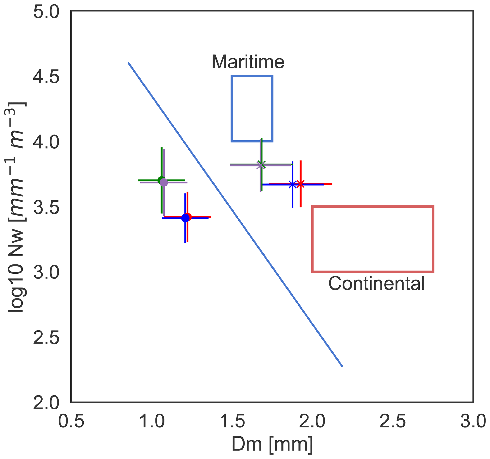
Figure 11Average values of log 10NW versus Dm for the data presented in this study (OTT1 in blue, OTT3 in red, T1 in green, T3 in purple) and their standard deviations. The blue line represents the demarcation between stratiform rainfall (dot points) (below the line) and convective rain (cross) (above the line), and each of the rectangles covers the clusters of data corresponding to maritime-like and continental-like as defined by Bringi et al. (2003) and augmented since by a number of authors such as Marzuki et al. (2013).
The potential sources and causes of errors and uncertainties that could explain observed differences between the instruments are discussed extensively in Angulo-Martinez et al. (2018), who also refer to previous work dedicated mostly to OTT Parsivel1,2. These authors list a number of possible causes, including the geometry of the laser beams, internal software differences, design of the mounting structure and brackets, a known underestimation of falling velocity for OTT Parsivel (Tokay et al., 2014). All of the above are likely contributing to cause most of the observed differences between the two types of instruments, but some of these issues will be challenging to solve, in particular in the absence of an independent absolute reference measurement of the DSD. High-frequency imagery (such as 2DVD disdrometers) has also been shown to have its own drawbacks and cannot be used as a reliable reference method, particularly for small diameters. Laser-based MPS has been hypothetically suggested as more reliable for measuring smaller drops (Thurai et al., 2017), but like other methods will remain subject to biases and errors. Overall, co-located measurements using different instrument types, such as Thurai et al. (2017), Angulo-Martinez et al. (2018) and the present work, are one of the possible ways of at least analysing the discrepancies between different measurement sources and discussing possible biases of each method, therefore providing a more robust estimate of the DSD spectra and derived integrated variables. In particular, such long-term high-resolution datasets are of importance for testing existing and new parameterisations of the DSD (Raupach et al., 2019; Thurai and Bringi, 2018; Thurai et al., 2019), combine weakness and strengths of each sensor to derive more accurate DSD spectra or investigate the sampling and spatio-temporal characteristics of rainfall at the micro scale (Uijlenhoet et al., 2003a, b, 2006; Jaffrain et al., 2011; Jaffrain and Berne, 2012a, b).
For the very first time, observations of the DSD have been presented for these temperate southern latitudes. In Australia, the only high-resolution DSD datasets have been obtained from experimental campaigns in the tropical north near Darwin (Maki et al., 2001; Giangrande et al., 2014), with only one short-term observation in subtropical Australia (Thurai et al., 2009). While the Southern Hemisphere in general lacks observations as compared to the Northern Hemisphere counterpart, Australia remains very poorly documented.
Figure 11 shows the observations of the mean DSD variables from this current work on the climate regime chart as presented in Bringi et al. (2003), also showing the continental-like and maritime-like clusters the authors identified based on the existing DSD observations. These observations with the Thies LPM always yielded higher NW and Dm as compared to the OTT Parsivel1, reflecting the larger number of smaller droplets as observed by the Thies LPM. If considering the Thies LPM data more complete because of including a larger portion of the full DSD spectra, this brings the current observations closer to the maritime-like cluster identified by Bringi et al. (2003). This is in agreement with the hypothesis of a larger number of small droplets generated in the precipitation originating from maritime environments.
This work presented for the very first time an open-access high-resolution PSVD dataset unique for this climate and location, including raw and carefully processed data with integrated DSD variables. This dataset could be further explored for a range of studies, such as the environmental factors that can contribute to the observed DSD characteristics, including diurnal precipitation type, seasonal and meso-scale precipitation variability, and the influence of oceanic or continental precipitation genesis. An obvious relevant future investigation given the main outcomes of this study would be the study of the effect of small diameter droplets (<0.6 mm) on integrated DSD variables and on the parameterisation of the DSD. As the present work has shown the capacity of the Thies LPM to capture this part of the drop size spectrum with high sensitivity, a study could build on this dataset and the recent findings from Thurai and Bringi (2018), Thurai et al. (2019) and Raupach et al. (2019) to study the parameterisation of the DSD, including the small droplets and the implication for retrievals such as Williams et al. (2014). Another direction of research could be the comparison of the Thies LPM to other instruments that unlike the OTT Parsivel1 or Parsivel2 are able to measure concentration of small droplets. Here, a new DSD dataset is provided for these latitudes and this climatic region, together with reflectivity–rainfall rate and attenuation–rainfall rate relationships, relevant for rainfall parameterisation and retrievals for ground- and satellite-based radars as well as microwave links. Lastly, similarly to other studies presenting co-located observations, this dataset gives the opportunity to study sampling effects and spatio-temporal characteristics of rainfall microphysics.
pyDSD and pyTmatrix (Leinonen, 2014) are openly available through GitHub repositories. We thank Joseph Hardin and Nick Guy for the development and freely available code of pyDSD (https://doi.org/10.5281/zenodo.9991; Hardin and Guy, 2017), which has been used in this study with modifications and further implementations for part of the processing.
The dataset presented in this study is publicly available at https://doi.org/10.5281/zenodo.3234218. This includes raw data for each of the four disdrometers (OTT1, OTT3, T1 and T3) recorded as daily “telegrams” by the in-built software of each instrument. Fields include the proprietary software-derived integrated variables and PSVD data.
Table A1Observation ranges of the Thies LPM and OTT Parsivel1 disdrometers for diameter and velocity bins.
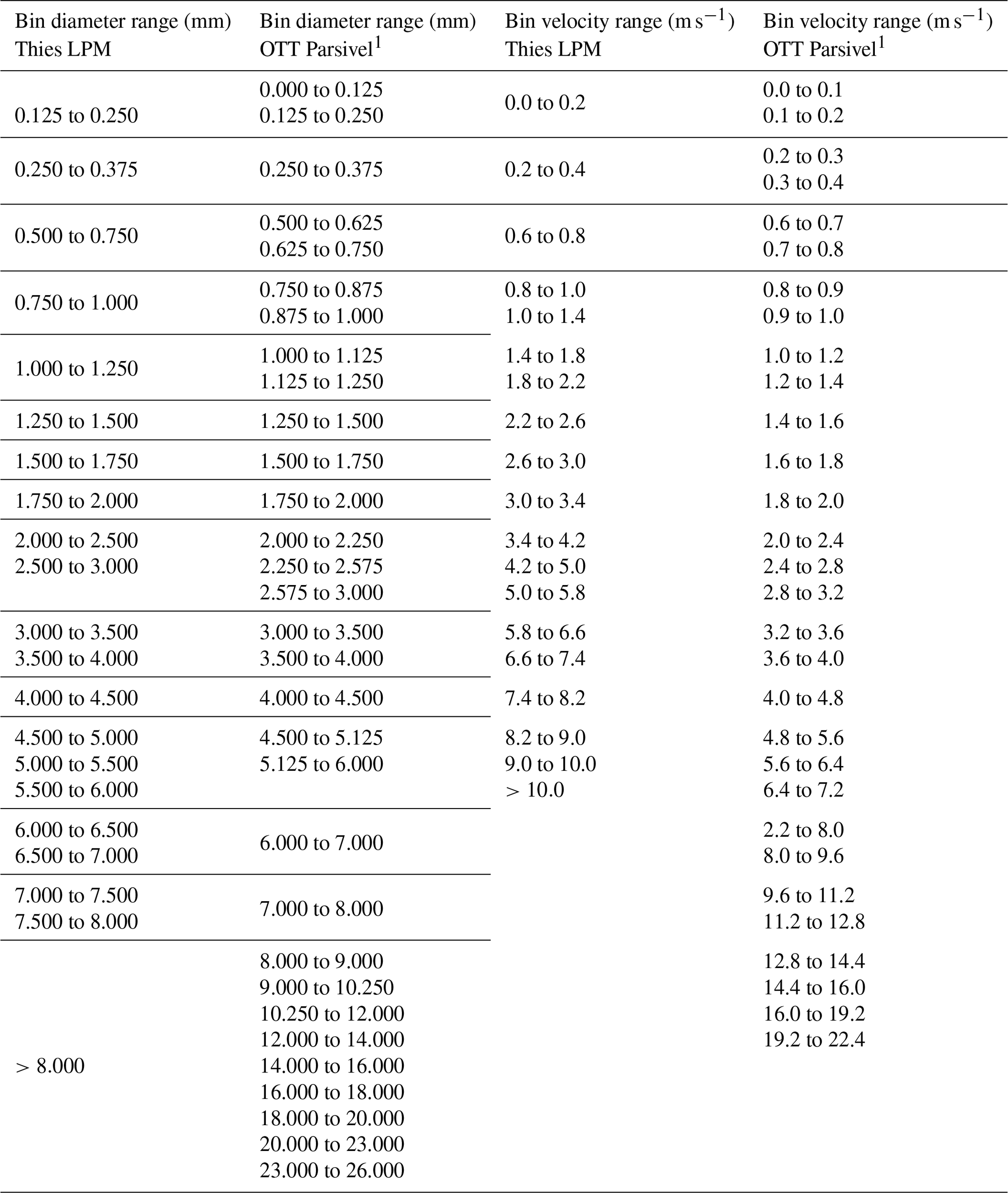
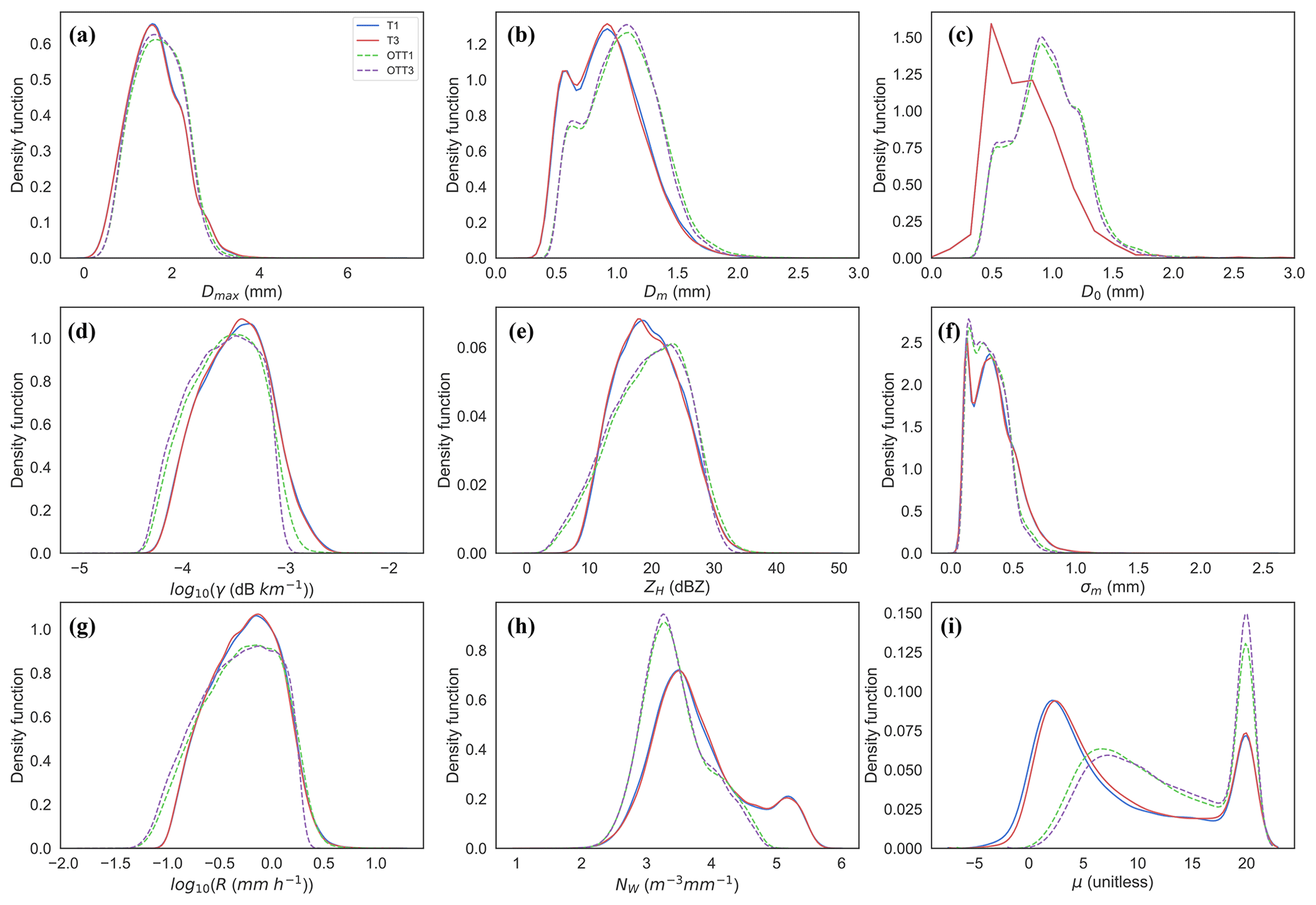
Figure A1Frequency plots of the DSD parameters, based on distributions (not shown) of integrated variables (Dmax, Dm, D0, γH, ZH, σm, R, NW and μ) for the four instruments (T1, T3, OTT1, OTT3) for rainfall rates of 0.1 to 2 mm h−1 (29 815 data points).
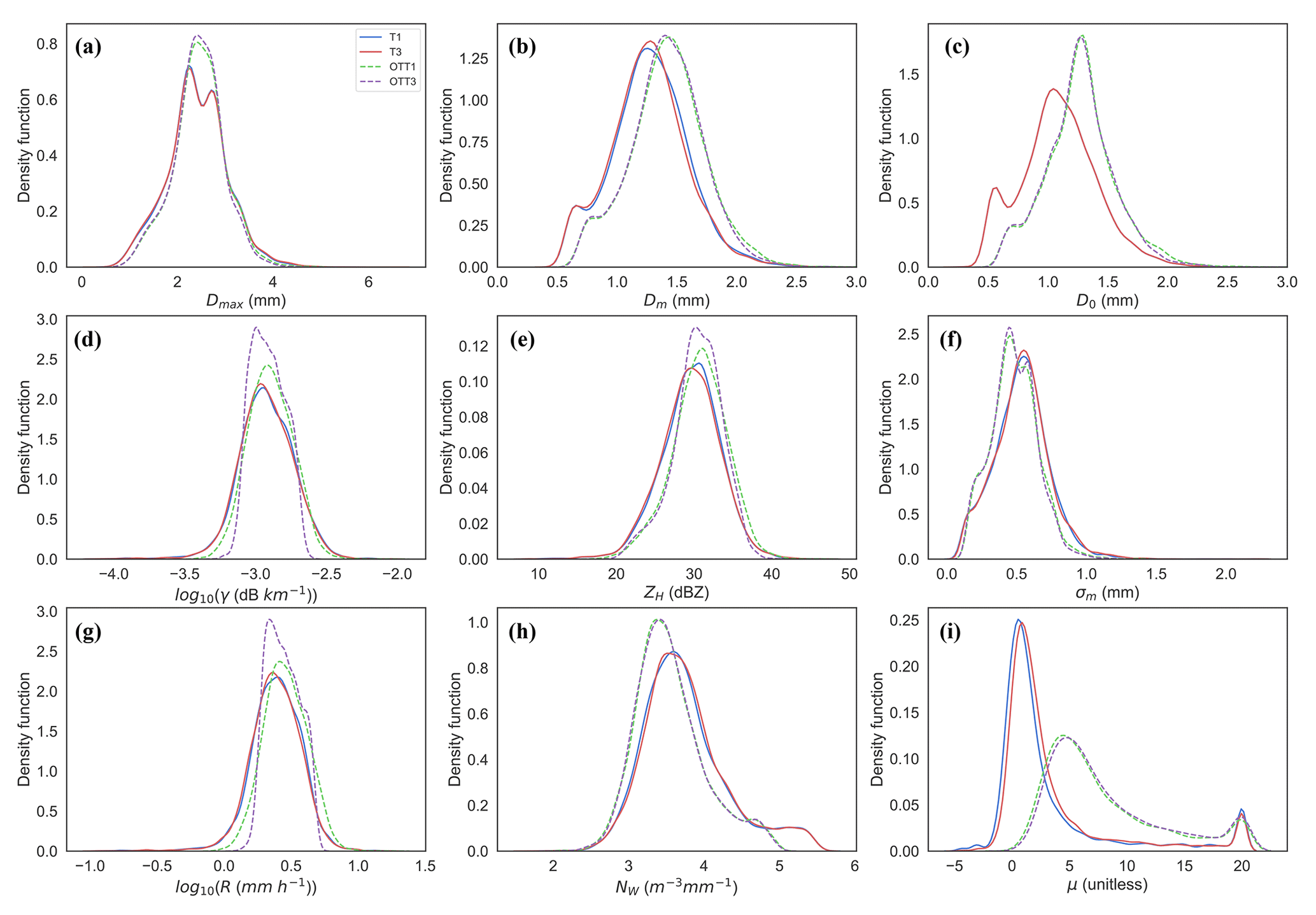
Figure A2Frequency plots of the DSD parameters, based on distributions (not shown) of integrated variables (Dmax, Dm, D0, γH, ZH, σm, R, NW and μ) for the four instruments (T1, T3, OTT1, OTT3) for rainfall rates of 2 to 5 mm h−1 (6967 data points).
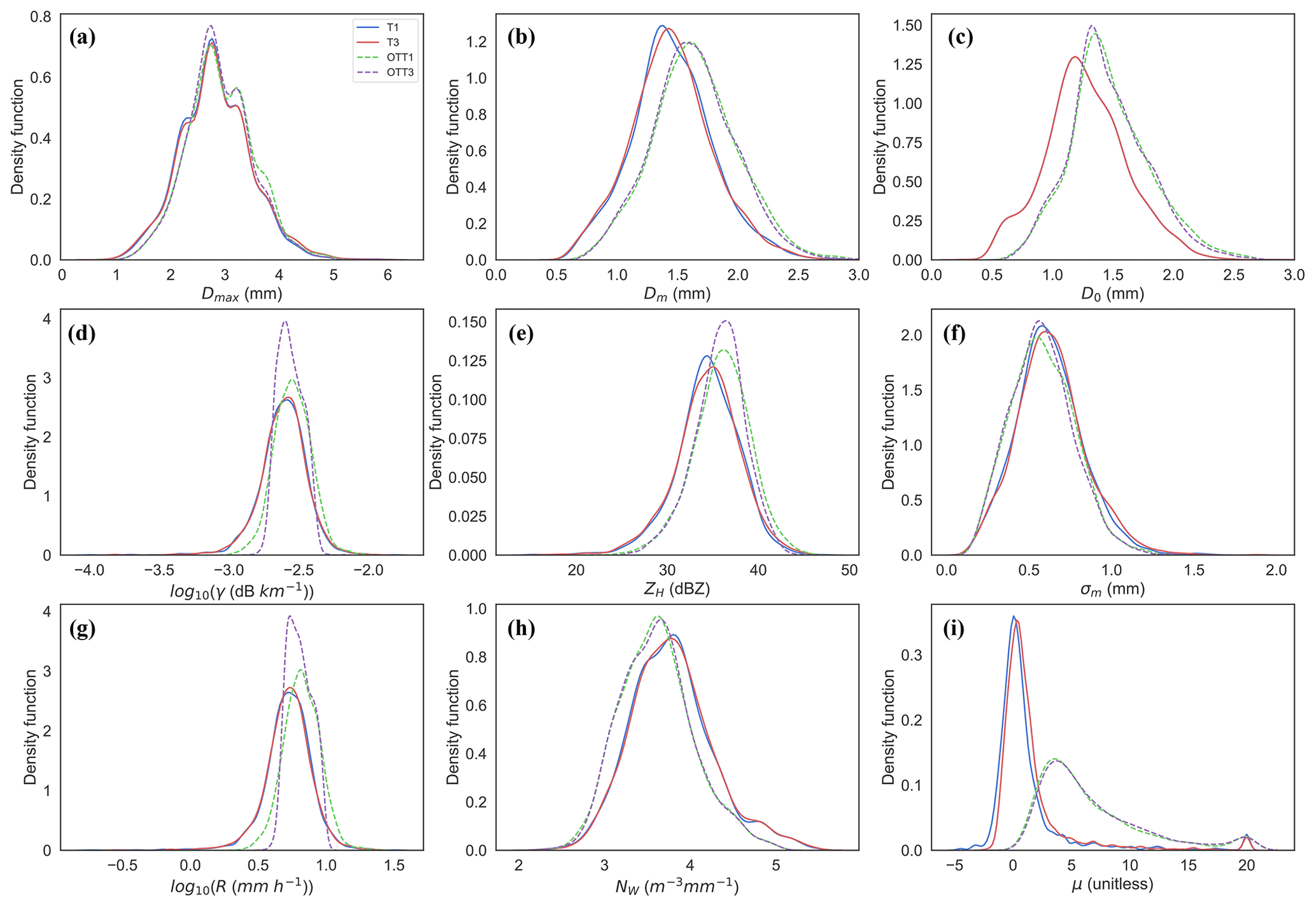
Figure A3Frequency plots of the DSD parameters, based on distributions (not shown) of integrated variables (Dmax, Dm, D0, γH, ZH, σm, R, NW and μ) for the four instruments (T1, T3, OTT1, OTT3) for rainfall rates of 5 to 10 mm h−1 (2398 data points).
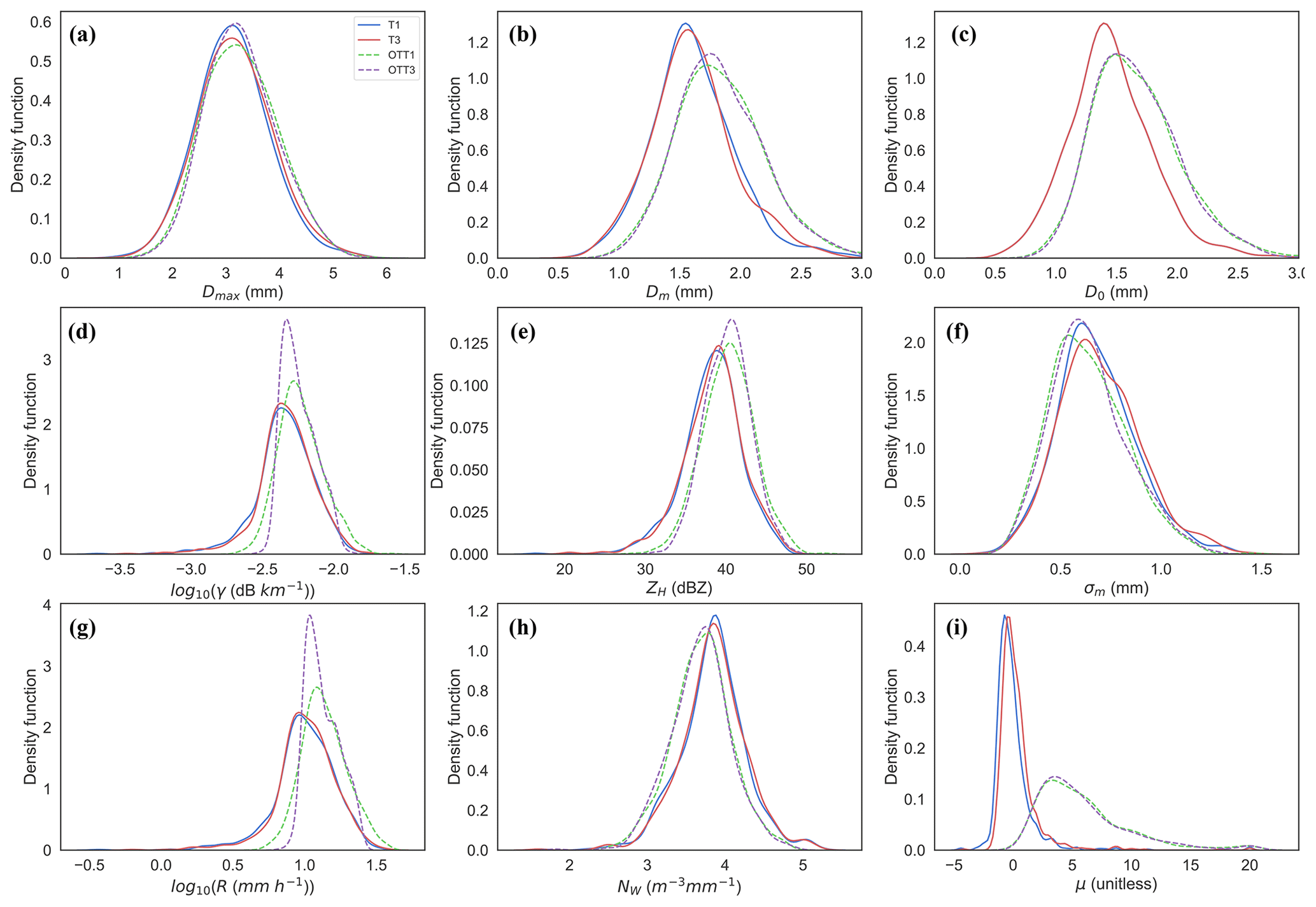
Figure A4Frequency plots of the DSD parameters, based on distributions (not shown) of integrated variables (Dmax, Dm, D0, γH, ZH, σm, R, NW and μ) for the four instruments (T1, T3, OTT1, OTT3) for rainfall rates of 10 to 25 mm h−1 (753 data points).
AG and JP developed the python pipeline to process the data built on top of existing pyDSD and pyTmatrix libraries. AG and JP performed the data analysis. All the co-authors provided ideas and feedback following discussions. AG prepared the manuscript with contributions from all the co-authors.
The authors declare that they have no conflict of interest.
The authors would like to thank the technical staff from the Australian Bureau of Meteorology (BoM) for the installation and maintenance of the disdrometers, in particular David Wright and Tom Kane. An Australian Research Council Discovery Project Grant number DP160101377 funded this project. Thanks to Valentin Louf for providing the suitable references for the observations of the DSD for the Darwin region. We thank the three anonymous reviewers for their insightful comments that helped improve the original submitted manuscript.
This research has been supported by the Australian Research Council (grant no. DP160101377).
This paper was edited by Matjaz Mikos and reviewed by three anonymous referees.
Adirosi, E., Roberto, N., Montopoli, M., Gorgucci, E., and Baldini, L.: Influence of Disdrometer Type on Weather Radar Algorithms from Measured DSD: Application to Italian Climatology, Atmosphere, 9, 360, https://doi.org/10.3390/atmos9090360, 2018.
Angulo-Martínez, M., Beguería, S., Latorre, B., and Fernández-Raga, M.: Comparison of precipitation measurements by OTT Parsivel2 and Thies LPM optical disdrometers, Hydrol. Earth Syst. Sci., 22, 2811–2837, https://doi.org/10.5194/hess-22-2811-2018, 2018.
Atlas, D., Srivastava, R. C., and Sekhon, R. S.: Doppler radar characteristics of precipitation at vertical incidence, Rev. Geophys., 11, 1–35, https://doi.org/10.1029/RG011i001p00001, 1973.
Battaglia, A., Rustemeier, E., Tokay, A., Blahak, U., and Simmer, C.: PARSIVEL Snow Observations: A Critical Assessment, J. Atmos. Ocean. Tech., 27, 333–344, https://doi.org/10.1175/2009JTECHA1332.1, 2010.
Baumgardner, D., Kok, G., Dawson, W., O'Connor, D., and Newton, R.: A new groundbased precipitation spectrometer: The Meteorological Particle Sensor (MPS), in: 11th Conf. on Cloud Physics, Ogden, UT, Amer. Meteor. Soc., 8.6, available at: https://ams.confex.com/ams/pdfpapers/ 41834.pdf (last access: 17 November 2019), 2002.
Beard, K. V.: Terminal velocity adjustment for cloud and precipitation drops aloft, J. Atmos. Sci., 34, 1293–1298, https://doi.org/10.1175/1520-0469(1977)034<1293:TVAFCA>2.0.CO;2, 1977.
Brandes, E. A., Zhang, G., and Vivekanandan, J.: Experiments in Rainfall Estimation with a Polarimetric Radar in a Subtropical Environment, J. Appl. Meteorol., 41, 674–685, https://doi.org/10.1175/1520-0450(2002)041<0674:EIREWA>2.0.CO;2, 2002.
Brawn, D. and Upton, G.: Estimation of an atmospheric gamma drop size distribution using disdrometer data, Atmos. Res., 87, 66–79, https://doi.org/10.1016/j.atmosres.2007.07.006, 2008.
Bringi, V. N., Chandrasekar, V., Hubbert, J., Gorgucci, E., Randeu, W. L., and Schoenhuber, M.: Raindrop Size Distribution in Different Climatic Regimes from Disdrometer and Dual-Polarized Radar Analysis, J. Atmos. Sci., 60, 354–365, https://doi.org/10.1175/1520-0469(2003)060<0354:RSDIDC>2.0.CO;2, 2003.
Chen, B., Wang, J., and Gong, D.: Raindrop size distribution in a midlatitude continental squall line measured by Thies optical disdrometers over East China, J. Appl. Meteorol. Clim., 55, 621–634, https://doi.org/10.1175/JAMC-D-15-0127.1, 2016.
Comstock, K. K., Wood, R., Yuter, S. E., and Bretherton, C. S.: Reflectivity and rain rate in and below drizzling stratocumulus, Q. J. Roy. Meteorol. Soc., 130, 2891–2918, https://doi.org/10.1256/qj.03.187, 2004.
de Moraes Frasson, R. P., da Cunha, L. K., and Krajewski, W. F.: Assessment of the Thies optical disdrometer performance, Atmos. Res., 101, 237–255, https://doi.org/10.1016/j.atmosres.2011.02.014, 2011.
Dolan, B., Rutledge, S. A., Lim, S., Chandrasekar, V., and Thurai, M.: A robust C-band hydrometeor identification algorithm and application to a long-term polarimetric radar dataset, J. Appl. Meteorol. Clim., 52, 2162–2186, https://doi.org/10.1175/JAMC-D-12-0275.1, 2013.
Fuchs, N. and Petrjanoff, I.: Microscopic examination of fog-, cloud- and rain droplets, Nature, 139, 111–112, 1937.
Giangrande, S. E., Bartholomew, M. J., Pope, M., Collis, S., and Jensen, M. P. A.: Summary of precipitation characteristics from the 2006–11 northern Australian wet seasons as revealed by ARM disdrometer research facilities (Darwin, Australia), J. Appl. Meteorol. Clim., 53, 1213–1231, https://doi.org/10.1175/JAMC-D-13-0222.1, 2014.
Hardin, J. and Guy, N.: PyDSD v1.0, https://doi.org/10.5281/zenodo.9991, 2017.
Illingworth, A. J. and Stevens, C. J.: An optical disdrometer for the measurement of raindrop size spectra in windy conditions, J. Atmos. Ocean. Tech., 4, 411–421, https://doi.org/10.1175/1520-0426(1987)004<0411:AODFTM>2.0.CO;2, 1987.
Islam, T., Rico-Ramirez, M. A., Han, D., and Srivastava, P. K.: A Joss–Waldvogel disdrometer derived rainfall estimation study by co-located tipping bucket and rapid response rain gauges, Atmos. Sci. Lett., 13, 139–150, https://doi.org/10.1002/asl.376, 2012.
ITU: Specific attenuation model for rain for use in prediction methods, Recommendation ITU-R P. 838, 3, available at: http://www.itu.int/dms_pubrec/itu-r/rec/p/r-rec-p.838-3-200503-i!!pdf-e.pdf (last access: 17 November 2019), 2005.
Jaffrain, J. and Berne, A.: Experimental quantification of the sampling uncertainty associated with measurements from PARSIVEL disdrometers, J. Hydrometeorol., 12, 352–370, https://doi.org/10.1175/2010JHM1244.1, 2011.
Jaffrain, J. and Berne, A.: Influence of the subgrid variability of the raindrop size distribution on radar rainfall estimators, J. Appl. Meteorol. Clim., 51, 780–785, https://doi.org/10.1175/JAMC-D-11-0185.1, 2012a.
Jaffrain, J. and Berne, A.: Quantification of the small-scale spatial structure of the raindrop size distribution from a network of disdrometers, J. Appl. Meteorol. Clim., 51, 941–953, https://doi.org/10.1175/JAMC-D-11-0136.1, 2012b.
Jaffrain, J., Studzinski, A., and Berne, A.: A network of disdrometers to quantify the small-scale variability of the raindrop size distribution, Water Resour. Res., 47, W00H06, https://doi.org/10.1029/2010WR009872, 2011.
Joss, J. and Waldvogel, A.: Ein spektrograph für niederschlagstropfen mit automatischer auswertung, Pure Appl. Geophys., 68, 240–246, https://doi.org/10.1007/BF00874898, 1967.
Joss, J. and Waldvogel, A.: Raindrop Size Distribution and Sampling Size Errors, J. Atmos. Sci., 26, 566–569, https://doi.org/10.1175/1520-0469(1969)026<0566:RSDASS>2.0.CO;2, 1969.
Kathiravelu, G., Lucke, T., and Nichols, P.: Rain drop measurement techniques: a review, Water, 8, 29, https://doi.org/10.3390/w8010029, 2016.
Klepp, C., Michel, S., Protat, A., Burdanowitz, J., Albern, N., Kähnert, M., Dahl, A., Louf, V., Bakan, S., and Buehler, S. A.: OceanRAIN, a new in-situ shipboard global ocean surface-reference dataset of all water cycle components, Scient. Data, 5, 180122, https://doi.org/10.1038/sdata.2018.122, 2018.
Krajewski, W. F. and Smith, J. A.: Radar hydrology: rainfall estimation, Adv. Water Resour., 25, 1387–1394, https://doi.org/10.1016/S0309-1708(02)00062-3, 2002.
Kruger, A. and Krajewski, W. F.: Two-Dimensional Video Disdrometer: A Description, J. Atmos. Ocean. Tech., 19, 602–617, https://doi.org/10.1175/1520-0426(2002)019<0602:TDVDAD>2.0.CO;2, 2002.
Leinonen, J.: High-level interface to T-matrix scattering calculations: architecture, capabilities and limitations, Opt. Express, 22, 1655–1660, https://doi.org/10.1364/OE.22.001655, 2014.
Louf, V., Protat, A., Warren, R. A., Collis, S. M., Wolff, D. B., Raunyiar, S., Jakob, C. and Petersen, W. A.: An Integrated Approach to Weather Radar Calibration and Monitoring Using Ground Clutter and Satellite Comparisons, J. Atmos. Ocean. Tech., 36, 17–39, https://doi.org/10.1175/JTECH-D-18-0007.1, 2019.
Mace, G. G. and Protat, A.: Clouds over the Southern Ocean as Observed from the R/V Investigator during CAPRICORN. Part I: Cloud Occurrence and Phase Partitioning, J. Appl. Meteorol., 57, 1783–1803, https://doi.org/10.1175/JAMC-D-17-0194.1, 2018a.
Mace, G. G. and Protat, A.: Clouds over the Southern Ocean as observed from the R/V Investigator during CAPRICORN. Part II: The properties of nonprecipitating stratocumulus, J. Appl. Meteorol. Clim., 57, 1805–1823, https://doi.org/10.1175/JAMC-D-17-0195.1, 2018b.
Maki, M., Keenan, T. D., Sasaki, Y., and Nakamura, K.: Characteristics of the raindrop size distribution in tropical continental squall lines observed in Darwin, Australia, J. Appl. Meteorol., 40, 1393–1412, https://doi.org/10.1175/1520-0450(2001)040<1393:COTRSD>2.0.CO;2, 2001.
Marshall, J. S. and Palmer, W. M.: The distribution of raindrops with size, J. Meteorol., 5, 165–166, 1948.
Marshall, J. S., Hitschfeld, W., and Gunn, K. L. S.: Advances in radar weather, Adv. Geophys., 2, 1–56, https://doi.org/10.1016/S0065-2687(08)60310-6, 1955.
Marzuki, M., Hashiguchi, H., Yamamoto, M. K., Mori, S., and Yamanaka, M. D.: Regional variability of raindrop size distribution over Indonesia, Ann. Geophys., 31, 1941–1948, https://doi.org/10.5194/angeo-31-1941-2013, 2013.
Merenti-Välimäki, H. L., Lönnqvist, J., and Laininen, P.: Present weather: comparing human observations and one type of automated sensor, Meteorol. Appl., 8, 491–496, 2001.
Moré, J. J.: The Levenberg-Marquardt algorithm: implementation and theory, in: Numerical analysis, Springer, Berlin, Heidelberg, 105–116, 1978.
Nawaby, A. S.: A method of direct measurement of spray droplets in an oil bath, J. Agr. Eng. Res., 15, 182–184, 1970.
Penide, G., Kumar, V. V., Protat, A., and May, P. T.: Statistics of drop size distribution parameters and rain rates for stratiform and convective precipitation during the north Australian wet season, Mon. Weather Rev., 141, 3222–3237, https://doi.org/10.1175/MWR-D-12-00262.1, 2013.
Petan, S., Rusjan, S., Vidmar, A., and Mikoš, M.: The rainfall kinetic energy–intensity relationship for rainfall erosivity estimation in the mediterranean part of Slovenia, J. Hydrol., 391, 314–321, https://doi.org/10.1016/j.jhydrol.2010.07.031, 2010.
Raupach, T. H. and Berne, A.: Correction of raindrop size distributions measured by Parsivel disdrometers, using a two-dimensional video disdrometer as a reference, Atmos. Meas. Tech., 8, 343–365, https://doi.org/10.5194/amt-8-343-2015, 2015.
Raupach, T. H., Thurai, M., Bringi, V. N., and Berne, A.: Reconstructing the Drizzle Mode of the Raindrop Size Distribution Using Double-Moment Normalization, J. Appl. Meteorol. Clim., 58, 145–164, https://doi.org/10.1175/JAMC-D-18-0156.1, 2019.
Sarkar, S., Phibbs, P., Simpson, R., and Wasnik, S.: The scaling of income distribution in Australia: Possible relationships between urban allometry, city size, and economic inequality, Environ. Plan. B, 45, 603–622, https://doi.org/10.1177/0265813516676488, 2018.
Sarkar, T., Das, S., and Maitra, A.: Assessment of different raindrop size measuring techniques: Inter-comparison of Doppler radar, impact and optical disdrometer, Atmos. Res., 160, 15–27, https://doi.org/10.1016/j.atmosres.2015.03.001, 2015.
Schönhuber, M., Lammer, G., and Randeu, W. L.: The 2D-Video-Distrometer, in: Precipitation: Advances in Measurement, Estimation and Prediction, edited by: Michaelides, S., Springer, Berlin, Heidelberg, 3–31, 2008.
Sheather, S. J. and Jones, M. C.: A reliable data-based bandwidth selection method for kernel density estimation, J. Roy. Stat. Soc. B, 53, 683–690, 1991.
Tapiador, F. J., Checa, R., and de Castro, M.: An experiment to measure the spatial variability of Rain Drop size distribution using sixteen laser disdrometers, Geophys. Res. Lett., 37, L16803, https://doi.org/10.1029/2010GL044120, 2010.
Testud, J., Oury, S., Black, R. A., Amayenc, P., and Dou, X.: The Concept of “Normalized” Distribution to Describe Raindrop Spectra: A Tool for Cloud Physics and Cloud Remote Sensing, J. Appl. Meteorol., 40, 1118–1140, https://doi.org/10.1175/1520-0450(2001)040<1118:TCONDT>2.0.CO;2, 2001.
Thompson, E. J., Rutledge, S. A., Dolan, B., Thurai, M., and Chandrasekar, V.: Dual-Polarization Radar Rainfall Estimation over Tropical Oceans, J. Appl. Meteorol. Clim., 57, 755–775, https://doi.org/10.1175/JAMC-D-17-0160.1, 2018.
Thurai, M. and Bringi, V. N.: Application of the generalized gamma model to represent the full rain drop size distribution spectra, J. Appl. Meteorol. Clim., 57, 1197–1210, https://doi.org/10.1175/jamc-d-17-0235.1, 2018.
Thurai, M., Bringi, V. N., and May, P. T.: Drop shape studies in rain using 2-D video disdrometer and dual-wavelength, polarimetric CP-2 radar measurements in south-east Queensland, Australia, in: Preprints, 34th Conf. on Radar Meteorology, Williamsburg, VA, 2009.
Thurai, M., Bringi, V. N., and May, P. T.: CPOL radar-derived drop size distribution statistics of stratiform and convective rain for two regimes in Darwin, Australia, J. Atmos. Ocean. Tech., 27, 932–942, https://doi.org/10.1175/2010JTECHA1349.1, 2010.
Thurai, M., Mishra, K. V., Bringi, V. N., and Krajewski, W. F.: Initial Results of a New Composite-Weighted Algorithm for Dual-Polarized X-Band Rainfall Estimation, J. Hydrometeorol., 18, 1081–1100, https://doi.org/10.1175/JHM-D-16-0196.1, 2017.
Thurai, M., Bringi, V., Gatlin, P. N., Petersen, W. A., and Wingo, M. T.: Measurements and Modeling of the Full Rain Drop Size Distribution, Atmosphere, 10, 39, https://doi.org/10.3390/atmos10010039, 2019.
Tokay, A., Petersen, W. A., Gatlin, P., and Wingo, M.: Comparison of raindrop size distribution measurements by co-located disdrometers, J. Atmos. Ocean. Tech., 30, 1672–1690, https://doi.org/10.1175/JTECH-D-12-00163.1, 2013.
Tokay, A., Wolff, D. B., and Petersen, W. A.: Evaluation of the new version of the laser-optical disdrometer, OTT Parsivel2, J. Atmos. Ocean. Tech., 31, 1276–1288, https://doi.org/10.1175/JTECH-D-13-00174.1, 2014.
Uijlenhoet, R. and Stricker, J. N. M.: A consistent rainfall parameterization based on the exponential raindrop size distribution, J. Hydrol., 218, 101–127, https://doi.org/10.1016/S0022-1694(99)00032-3, 1999.
Uijlenhoet, R.: Raindrop size distributions and radar reflectivity–rain rate relationships for radar hydrology, Hydrol. Earth Syst. Sci., 5, 615–628, https://doi.org/10.5194/hess-5-615-2001, 2001.
Uijlenhoet, R. and Sempere Torres, D.: Measurement and parameterization of rainfall microstructure, J. Hydrol., 328, 1–7, https://doi.org/10.1016/j.jhydrol.2005.11.038, 2006.
Uijlenhoet, R., Smith, J. A., and Steiner, M.: The microphysical structure of extreme precipitation as inferred from ground-based raindrop spectra, J. Atmos. Sci., 60, 1220–1238, https://doi.org/10.1175/1520-0469(2003)60<1220%3ATMSOEP>2.0.CO%3B2, 2003a.
Uijlenhoet, R., Steiner, M., and Smith, J. A.: Variability of raindrop size distributions in a squall line and implications for radar rainfall estimation, J. Hydrometeorol., 4, 43–61, https://doi.org/10.1175/1525-7541(2003)004<0043:VORSDI>2.0.CO;2, 2003b.
Uijlenhoet, R., Porrà, J. M., Sempere-Torres, D., and Creutin, J.-D.: Analytical solutions to sampling effects in drop size distribution measurements during stationary rainfall: Estimation of bulk rainfall variables, J. Hydrol., 328, 65–82, https://doi.org/10.1016/j.jhydrol.2005.11.043, 2006.
Ulbrich, C. W.: Natural Variations in the Analytical Form of the Raindrop Size Distribution, J. Clim. Appl. Meteorol., 22, 1764–1775, https://doi.org/10.1175/1520-0450(1983)022<1764:NVITAF>2.0.CO;2, 1983.
Ulbrich, C. W. and Atlas, D.: Rainfall Microphysics and Radar Properties: Analysis Methods for Drop Size Spectra, J. Appl. Meteorol., 37, 912–923, https://doi.org/10.1175/1520-0450(1998)037<0912:RMARPA>2.0.CO;2, 1998.
Vali, G., Kelly, R. D., French, J., Haimov, S., Leon, D., McIntosh, R. E., and Pazmany, A.: Finescale structure and microphysics of coastal stratus, J. Atmos. Sci., 55, 3540–3564, https://doi.org/10.1175/1520-0469(1998)055<3540:FSAMOC>2.0.CO;2, 1998.
Verdon-Kidd, D. C. and Kiem, A. S.: On the relationship between large-scale climate modes and regional synoptic patterns that drive Victorian rainfall, Hydrol. Earth Syst. Sci., 13, 467–479, https://doi.org/10.5194/hess-13-467-2009, 2009.
Williams, C. R., Bringi, V. N., Carey, L. D., Chandrasekar, V., Gatlin, P. N., Haddad, Z. S., Meneghini, R., Joseph Munchak, S., Nesbitt, S. W., Petersen, W. A., Tanelli, S., Tokay, A., Wilson, A., and Wolff, D. B.: Describing the Shape of Raindrop Size Distributions Using Uncorrelated Raindrop Mass Spectrum Parameters, J. Appl. Meteorol. Clim., 53, 1282–1296, https://doi.org/10.1175/JAMC-D-13-076.1, 2014.