the Creative Commons Attribution 4.0 License.
the Creative Commons Attribution 4.0 License.
 | 28 Jan 2019
Subseasonal hydrometeorological ensemble predictions in small- and medium-sized mountainous catchments: benefits of the NWP approach
Massimiliano Zappa
Christoph Spirig
Christoph Schär
Konrad Bogner
Traditional ensemble streamflow prediction (ESP) systems are known to provide a valuable baseline to predict streamflows at the subseasonal to seasonal timescale. They exploit a combination of initial conditions and past meteorological observations, and can often provide useful forecasts of the expected streamflow in the upcoming month. In recent years, numerical weather prediction (NWP) models for subseasonal to seasonal timescales have made large progress and can provide added value to such a traditional ESP approach. Before using such meteorological predictions two major problems need to be solved: the correction of biases, and downscaling to increase the spatial resolution. Various methods exist to overcome these problems, but the potential of using NWP information and the relative merit of the different statistical and modelling steps remain open. To address this question, we compare a traditional ESP system with a subseasonal hydrometeorological ensemble prediction system in three alpine catchments with varying hydroclimatic conditions and areas between 80 and 1700 km2. Uncorrected and corrected (pre-processed) temperature and precipitation reforecasts from the ECMWF subseasonal NWP model are used to run the hydrological simulations and the performance of the resulting streamflow predictions is assessed with commonly used verification scores characterizing different aspects of the forecasts (ensemble mean and spread). Our results indicate that the NWP-based approach can provide superior prediction to the ESP approach, especially at shorter lead times. In snow-dominated catchments the pre-processing of the meteorological input further improves the performance of the predictions. This is most pronounced in late winter and spring when snow melting occurs. Moreover, our results highlight the importance of snow-related processes for subseasonal streamflow predictions in mountainous regions.
- Article
(6099 KB) -
Supplement
(1973 KB) - BibTeX
- EndNote


Subseasonal hydrometeorological predictions are of special interest for many different applications in the public and private sectors, for example, to develop early warning systems for flood and drought preparedness for the general public (Bogner et al., 2018; Cloke and Pappenberger, 2009; Fundel et al., 2013; Van Lanen et al., 2016; Schär et al., 2004; White et al., 2017), to optimize the production of renewable energy sources such as wind (Beerli et al., 2017), solar (Inman et al., 2013), and hydro power (García-Morales and Dubus, 2007), or to ensure inland waterway transportation (Meißner et al., 2017).
In recent years the numerical weather prediction (NWP) systems have greatly evolved (Bauer et al., 2015). The ensemble forecasting approach introduced 2 decades ago allows the chaotic nature of the atmosphere to be captured in a probabilistic sense and has extended the horizon to which weather predictions can provide valuable information. Hydrological prediction systems, especially beyond the short-range lead times, benefit from such an ensemble approach (Demargne et al., 2014; Jaun et al., 2008; Schaake et al., 2007; Verbunt et al., 2007). Ensemble hydrometeorological end-to-end prediction systems for the subseasonal timescale, i.e. forecasts for lead times up to 4 to 6 weeks, are now being developed and investigated for different parts in the world. Nowadays, different research initiatives (Hao et al., 2018; Robertson et al., 2015; Vitart et al., 2017; Vitart and Robertson, 2018) set their focus on the assessment of predictability within this lead-time horizon. But still this lead time between the medium-range forecasts and the seasonal predictions is a grey zone in both the meteorological and hydrological forecasting communities.
However, ensemble prediction systems have extensively been used for short- to medium-range forecasts and it could be shown that the resolution of the model plays an important role for a good performance of ensemble precipitation forecasts (Marsigli et al., 2008; Montani et al., 2001, 2003). A higher resolution can be achieved by dynamically downscaling the ensemble predictions, which led to a gain in predictability in ensemble precipitation forecast over the past years in the medium-range timescale (Montani et al., 2011). From a hydrological perspective flood peaks can much better be predicted using mesoscale ensemble forecast models compared to global models (Davolio et al., 2012). In such operational short- to medium-range forecasting systems, dynamical downscaling methods are a valuable tool to increase the resolution of the forecasts, but for long-term predictions the computational demand of dynamical downscaling methods is a limiting factor, and it has been shown that similar results can be achieved with statistical downscaling methods (Díez et al., 2005; Manzanas et al., 2018). In recent years, seasonal ensemble prediction systems have increasingly been used in the hydrological forecasting context. At this timescale downscaling is usually included in statistical processing techniques that primarily aim at correcting the bias of the meteorological forecast. Different statistical bias correction techniques can be used to improve the skill of seasonal forecasts (Bohn et al., 2010; Crochemore et al., 2016; Kumar et al., 2014). An alternative approach for seasonal streamflow prediction is the traditional ensemble prediction system (ESP) first introduced by Day (1985). In this approach, observed historical meteorological conditions are used to generate the streamflow forecasts. Several studies have shown that ESP can provide skilful seasonal streamflow prediction (Harrigan et al., 2018) and seasonal hydrometeorological prediction systems have difficulties in outperforming the ESP beyond a 1-month lead time (Arnal et al., 2018; Lucatero et al., 2018b). Irrespective of the methodology used, the performance of ensemble streamflow forecasts depends to a large degree on the initial condition within the catchment, especially for small catchments (Van Dijk et al., 2013; Thirel et al., 2010). In subseasonal to seasonal hydrometeorological predictions, the memory of the river networks is predominately driven by the initial conditions of the land surface characteristics, i.e. soil moisture and snow cover (Jörg-Hess et al., 2015a). It has been shown that these parameters play an important role for skilful hydrometeorological forecasts using NWP inputs in hydrological models for streamflow forecasting (Orth and Seneviratne, 2013b; Sinha and Sankarasubramanian, 2013). However, for small snow-dominated catchments the benefit of using pre-processed subseasonal NWP input has not yet been investigated. The three main reasons for the lack of studies at smaller scales is the fact that the driving meteorological models are calculated on a global scale with coarse resolution. Therefore, small catchments are often smaller than the nominal resolution of these models, making a pre-processing step necessary to bias-correct and downscale the meteorological forecasts to an adequate spatial resolution as an input to the hydrological models. The second reason is that small catchments usually do not have a long temporal memory and processes leading to runoff are rather quick and therefore the skill in early lead times does not extend into longer lead times (Orth and Seneviratne, 2013a). As a consequence, the upper limits of the forecast skill at the subseasonal timescale strongly depend on such catchment characteristics (Bogner et al., 2016, 2018). Finally, previous generations of subseasonal to seasonal climate forecasts rapidly lost skill beyond the first 2 weeks (see for example Lavers et al., 2009).
Small- and medium-sized catchments in mountainous regions such as the Alps are often snow dominated; hence the streamflow, and especially the forecasts thereof, depend to a large degree on snowmelt processes that are driven by temperature (Hock, 2003; Ohmura, 2001; Zappa et al., 2003). Monhart et al. (2018) have shown that the statistically corrected subseasonal temperature forecasts exhibit positive skill compared to the climatological reference of up to 3 weeks, whereas positive skill of precipitation forecasts is restricted to the first 10 days. Hence, the question arises whether and to what extent the positive skill of temperature forecasts in meteorological prediction models further progresses to the streamflow forecasts. Skilful streamflow forecasts might not directly be related to the skill in temperature forecasts but rather in an appropriate sampling of the initial conditions and the actual snow cover (snow water equivalent) at initialization (Jörg-Hess et al., 2015a). Therefore, the skill of the streamflow forecasts will not solely depend on the quality of temperature forecasts alone. To investigate this question, ensemble streamflow prediction can be used to evaluate the importance of the initial conditions. The comparison of the skill of an ESP forecast and the skill of actual hydrometeorological predictions can indicate the relative importance of using physically consistent meteorological forecasts to produce skilful streamflow predictions. After presenting the methods used for the pre-processing and the verification of the different forecasts in Sect. 2, the meteorological and hydrological data are described in Sect. 3. The results obtained are presented in detail in Sect. 4 and followed by a discussion (Sect. 5) to put the results in the current scientific context.
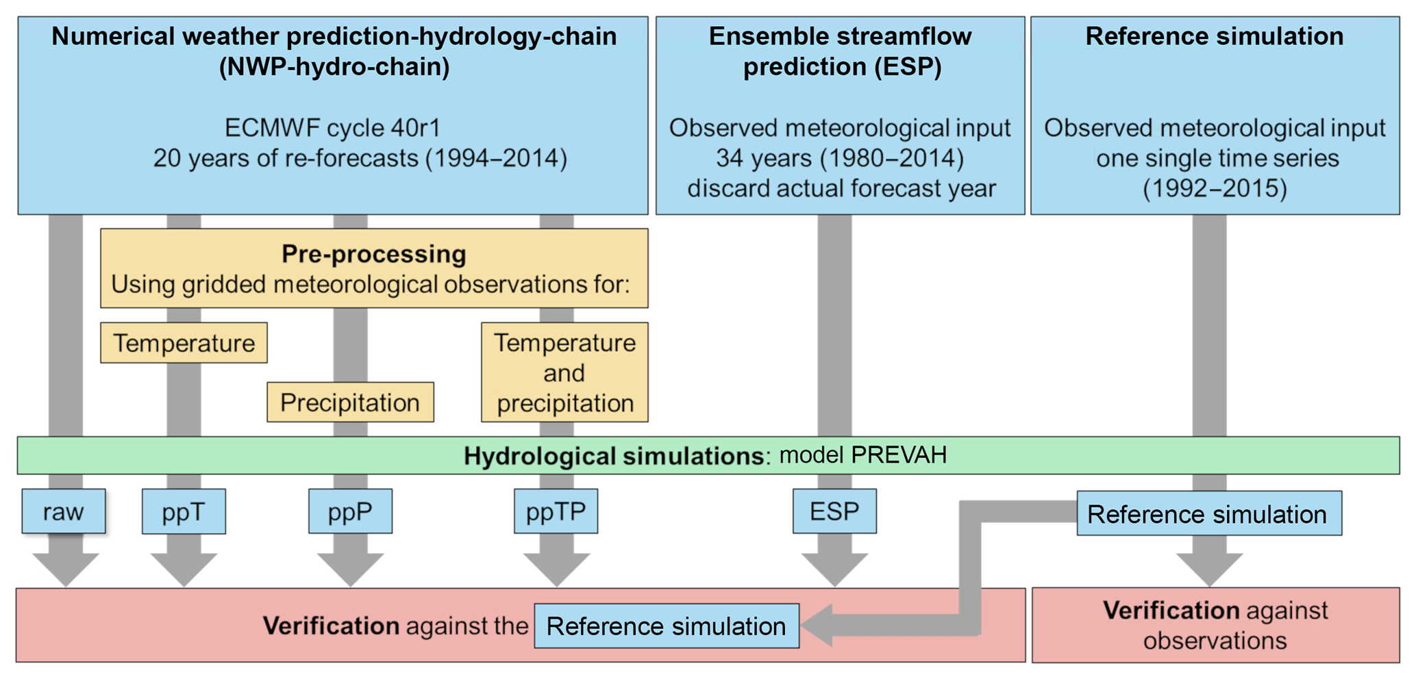
Figure 1Conceptual design of the NWP-Hydro-chain with and without pre-processing (left) and the ESP chain (right).
The conceptual framework used in this study is presented in Fig. 1. The hydrological model is run with different meteorological forcings to provide ensemble streamflow predictions. A traditional ESP approach using 34 years of meteorological observations provides the baseline forecasts. A second input is based on the reforecasts from the ECMWF subseasonal prediction system as described in Sect. 3.1. Along this chain four different configurations are used to feed the hydrological model and generate streamflow predictions: the raw reforecasts for both temperature and precipitation, the raw precipitation reforecast and pre-processed temperature reforecasts and vice versa, and both parameters pre-processed.
2.1 Pre-processing in the hydrometeorological model chain
In the pre-processing step a quantile mapping (QM) technique is applied in a leave-one-year-out set-up to correct each re-forecast year separately. The corrections are applied in a lead-time-dependent manner. A description of the pre-processing set-up can be found in Monhart et al. (2018). This cross-calibration framework ensures a cross-validation described in Sect. 2.3. In contrast to the site-specific pre-processing set-up used in Monhart et al. (2018), a gridded observational product is used here. The pre-processing is performed for temperature and precipitation and involves not only a bias correction, but also a downscaling because of the higher resolution of the gridded observation data used in this study. The observation and forecast data used in this study are described in more detail in Sect. 3. However, it is worth mentioning here that the raw model resolution of 50 km is bias corrected with QM using gridded observations with a higher spatial resolution of 2 km. This resolution corresponds to the meteorological input of the hydrological model, for which observations from station data are interpolated to 2 km grids (see Sect. 3.2). The QM technique is a simple and widely used method for pre-processing hydrometeorological forecasts (e.g. Kang et al., 2010; Lucatero et al., 2018b; Verkade et al., 2013). For a given target day of a reforecast the correction is derived from the distribution of all the reforecasts within a 3-week window around the same lead day and the corresponding observations; hence, the correction depends on both the lead time and the period of the years. For temperature an additive correction and for precipitation a multiplicative correction is applied. Using the multiplicative version of QM for temperature allows us to include zero value without special treatment. Hence, no precipitation can be generated if the raw forecasts do not exhibit any rain.
2.2 ESP
The ensemble streamflow predictions follow the established procedure first proposed by Day (1985). Many studies have shown the potential of this method to provide skilful streamflow predictions at the subseasonal to seasonal timescale in Europe (e.g. Arnal et al., 2018; Harrigan et al., 2018). The basic principle behind the ESP is to create an ensemble of streamflows based on known initial conditions and forced by historic climate sequences. The historical record used in this study covers the period from 1980 to 2014, resulting in 34 members for each forecast. As in the hydrometeorological model chain, the ESP approach is set up in a leave-one-year-out manner to ensure that the information of the year to be verified is not part of the forecasts itself. ESPs can be skilful especially in catchments where the predictability is mainly driven by the initial conditions, although the quality of the predictions depends on the seasons and hydroclimatic characteristics (Wood and Lettenmaier, 2008).
2.3 Hydrological simulations
The hydrological simulations are performed with the Precipitation-Runoff-Evapotranspiration-Hydrotope model (PREVAH) (Gurtz et al., 1999; Viviroli et al., 2009a; Zappa et al., 2003). In this study, the distributed model version which requires gridded input data is used as described in Speich et al. (2015) and first applied in a hydrological study by Schattan et al. (2013). The model requires spatial information (land use, aspect, and elevation) and gridded meteorological variables. Besides the statistically corrected temperature and precipitation predictions, relative humidity, sunshine duration, surface albedo, and solar radiation are needed to run PREVAH. For the initialization of the model the required fields (i.e. soil moisture, groundwater storages, snow cover) are used from a reference simulation driven with the gridded meteorological observation dataset as described in Sect. 3.4. The distributed hydrological model is run at a resolution of 200 m × 200 m; hence, the same model-internal procedures are used to further downscale the meteorological inputs for all different experiments. Namely, an interpolation based on inverse distance weighting (IDW) and different height- and terrain-specific corrections are applied to the input variables (adiabatic lapse rate correction; aspect and slope corrections) as described in Zappa et al. (2003). A more extensive description of the model and a comparison to the HRU-based version of the model can be found in Jörg-Hess et al. (2015a).
2.4 Verification
To verify the predictions, various metrics are used to assess the forecast performance according to different characteristics or attributes of the forecasts respectively. The verification is performed for the two variables streamflow and snow water equivalent (SWE). For the selection of verification metrics we follow the procedures presented in Brown et al. (2010) and we combine deterministic and probabilistic measures of skill to assess the forecast performance. More detailed reviews of ensemble forecast verification can be found in Jolliffe and Stephenson (2012) and Wilks (2011). Besides the Nash–Sutcliffe efficiency (NSE) (Nash and Sutcliffe, 1970) widely used to assess the performance of hydrological models and the logarithmic version thereof (NSE log), which is more sensitive to low flows (Krause et al., 2005), we use the ensemble mean error (bias) and the mean absolute error (MAE). For both versions of the NSE and the bias the ensemble mean is used for the calculation. Although these metrics can describe the average characteristics of the ensemble forecasts, it has been shown that it is crucial to consider the spread of the ensemble forecast as well to properly assess the forecast performance in particular at the subseasonal to seasonal timescale (Kumar et al., 2014). Therefore the continuous ranked probability skill score (CRPSS) with the extension proposed by Ferro (2014) to account for small ensemble sizes is used to characterize the performance of the full ensemble (Hersbach, 2000; Müller et al., 2005). In addition, we use the spread-to-error ratio (SprErr) as an indicator of the forecast reliability (Hopson, 2014). The SprErr is defined as the ratio between the variance of the forecast ensemble (forecast spread) and the mean squared error (MSE) of the ensemble forecast (forecast error). For reliable forecasts the spread and the error are equal, resulting in a SprErr of 1, whereas values below 1 indicate overconfidence (errors are larger compared to the spread) and values above 1 indicate overdispersion (the spread is larger compared to the error). Finally, rank histograms are used to visually examine the reliability of the forecasts (Anderson, 1996; Talagrand et al., 1997; Hamill and Colucci, 1997). In each of these scores the reforecasts are compared to observations (ME and MAE) and the climatology of the reference simulation is used as a reference climatology for NSE and CRPSS. In this study we use pseudo observations from a reference simulation to substitute real observations for the streamflow forecast verification. This is done to separate the effect on the performance of the hydrological predictions resulting either from different meteorological input forecasts or from the deficits in the hydrological model in simulating low flows. The set-up of the reference simulation to generate the pseudo observations is described in data Sect. 3.4.
3.1 Meteorological reforecast data
We obtained the subseasonal reforecasts from ECMWF Integrated Forecasting System (IFS) version CY40r1. This version was operational from 19 November 2013 to 12 May 2015. This is a unique dataset because no system change occurred for nearly 1.5 years (http://www.ecmwf.int/en/forecasts/documentation-and-support/changes-ecmwf-model/cycle-40r1/cycle-40r1, last access: 1 August 2018, for the documentation of IFS CY40r1). Routinely the model is updated more frequently within 1 year and therefore changes in the system, e.g. changes to the horizontal and vertical resolution or changes in the parametrization of physical processes, affect the skill of the forecast over the course of the year. The same dataset is used as in the study presented by Monhart et al. (2018) and can be referred to for a more detailed description of the forecast system and for an extensive verification of these meteorological forecasts.
In this study the historical five-member reforecasts (i.e. hindcasts) are used to drive the hydrological simulations. These meteorological reforecasts are run for all forecasts issued on Thursdays using ERA-Interim analysis for the initialization (ECMWF, 2014) covering the period from April 1994 to March 2014, resulting in a total of 1040 individual reforecasts that are analysed within this study. These reforecasts are essential for the post-processing of the meteorological forecasts (i.e. pre-processing from a hydrological point of view). The bias of the forecasting system can be estimated using the reforecasts and future forecasts can be corrected (or, as in this analysis, the reforecasts themselves).
3.2 Meteorological observational data
We use gridded observation datasets at 2 km × 2 km resolution for daily temperature and precipitation to pre-process the meteorological reforecasts and for the verification thereof (Frei, 2014; Isotta et al., 2014; Meteoswiss, 2016a, b). These products are based on surface observations and are often used in climatological studies for Switzerland (e.g. Addor et al., 2016; Begert and Frei, 2018, Orth et al., 2015 for a hydrological model study with the same model version we use in this study). Nevertheless such gridded observational products exhibit limitations especially in complex terrain with high mountain peaks because of the interpolation errors and errors induced by natural variability (Frei, 2014; Addor and Fischer, 2015). Despite these limitations the analysis benefits by using the gridded version because of the scarcity of meteorological stations available in the catchment areas. The additional meteorological variables (relative humidity, sunshine duration, surface albedo and solar radiation) needed to run the PREVAH hydrological model are directly used from the (raw) meteorological forecasts and are inherently downscaled with the PREVAH internal methodology. Although these parameters could influence the hydrological relevant processes, e.g. evaporation rates from snow based on the relative humidity which could change after a downscaling, a thorough assessment of the effect of bias correcting and downscaling of these additional variables is out of scope of the current study.
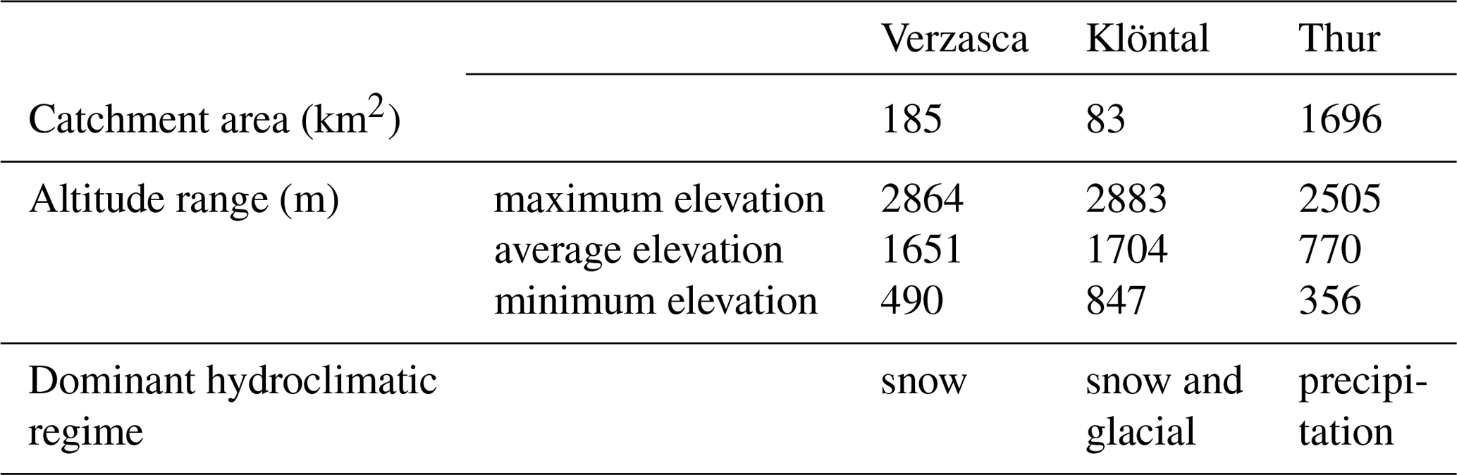
Table 1Overview of the catchment characteristics for the three catchments analysed.
3.3 Catchment characteristics and hydrological data
The experiments analysed in this study are performed for three alpine catchments with various hydro-climatic characteristics. This allows identification of the underlying processes that lead to skilful subseasonal streamflow predictions. The selection of the catchments is a compromise between the intended applications of our results within hydropower optimization in the Alpine region and adequately meeting the requirements of a scientific analysis. Hence, the Klöntal and the Verzasca catchment both are selected because of existing hydropower installations in these watersheds and the Thur catchment was chosen as a representative catchment with different hydroclimatic characteristics and because this catchment is often considered in hydrological research in Switzerland. An overview of the catchment characteristics can be found in Table 1.
The Verzasca catchment located in the southern part of the Alps is snow dominated in the cold seasons and more precipitation dominated in warm seasons (Wöhling et al., 2006). The average height of the catchment is 1651 m a.s.l. with a maximum height of 2864 m a.s.l. and a minimum height at the gauging station of 490 m a.s.l. Despite this height difference the catchment is of medium size only, with a total of 185 km2. The runoff in this catchment is low in winter due to accumulation of snow in elevated regions and highly dynamical in late spring to early autumn because the area is prone to heavy thunderstorm activity (Bogner et al., 2018; Liechti et al., 2013). The data used for calibration of the hydrological model and for the verification of the reference simulation are provided by the Federal Office for the Environment (FOEN) for the Lavertezzo gauging station.
The Klöntal catchment, located in the northern part of the Alps, is mainly snow dominated and inherits a glaciated area of about 3 km2 (<5 %). The maximum height is 2883 m a.s.l. and the minimum height, corresponding to the height of Lake Klöntal, is 847 m a.s.l. with a catchment area of 83 km2 categorized as a small catchment. The lake is used for hydropower generation. The data provided by the hydropower operator are used for calibration of the hydrological model and the verification of the streamflow reforecasts. Due to the absence of gauging stations, these data are an estimate of the streamflow at the lake outlet and deduced from the water balance of historical lake levels. Hence, the quality of the data is lower compared to the other two catchments, and therefore the interpretation especially under low-flow conditions should be treated with care.
The third catchment under investigation is the pre-alpine Thur catchment. This catchment is of medium size with 1696 km2 and mainly precipitation dominated. The highest elevation is 2505 m, the lowest elevation at the gauging station in Andelfingen provided by the FOEN is 356 m, and the mean catchment height is 770 m a.s.l. This catchment has frequently been analysed in the literature (Bogner et al., 2016; Fundel et al., 2013; Jörg-Hess et al., 2015b).
3.4 Hydrological pseudo observations: the reference simulation
For all three catchments described above, the reference simulation is generated using an observed gridded meteorological dataset for the meteorological variables (temperature, precipitation, relative humidity, sunshine duration, surface albedo, and solar radiation) to run the PREVAH hydrological model (see Sect. 2.3) in the same setting as used for different previous studies (Orth et al., 2015; Schattan et al., 2013; Speich et al., 2015). The gridding of all the meteorological variables makes use of elevation-based de-trending and inverse-distance-based interpolation as detailed in the baseline publication on PREVAH and its tools (Viviroli et al., 2009a) and also used for application of other hydrological models (e.g. Melsen et al., 2016). The reference simulation is a single time series starting in 1992 (after a spin-up period of 3 years) and ending in 2015. The spin-up period ensures the stability of the streamflow simulations and is of particular importance to fill low-frequency storages for baseflow and snow (Viviroli et al., 2009b). In addition the spin-up times highly vary across catchments depending on the hydroclimatic characteristics and catchment size (Rahman et al., 2016; Seck et al., 2015). The climatology of the reference simulation is referred to as the reference climatology and is used as a reference for the computation of skill scores.
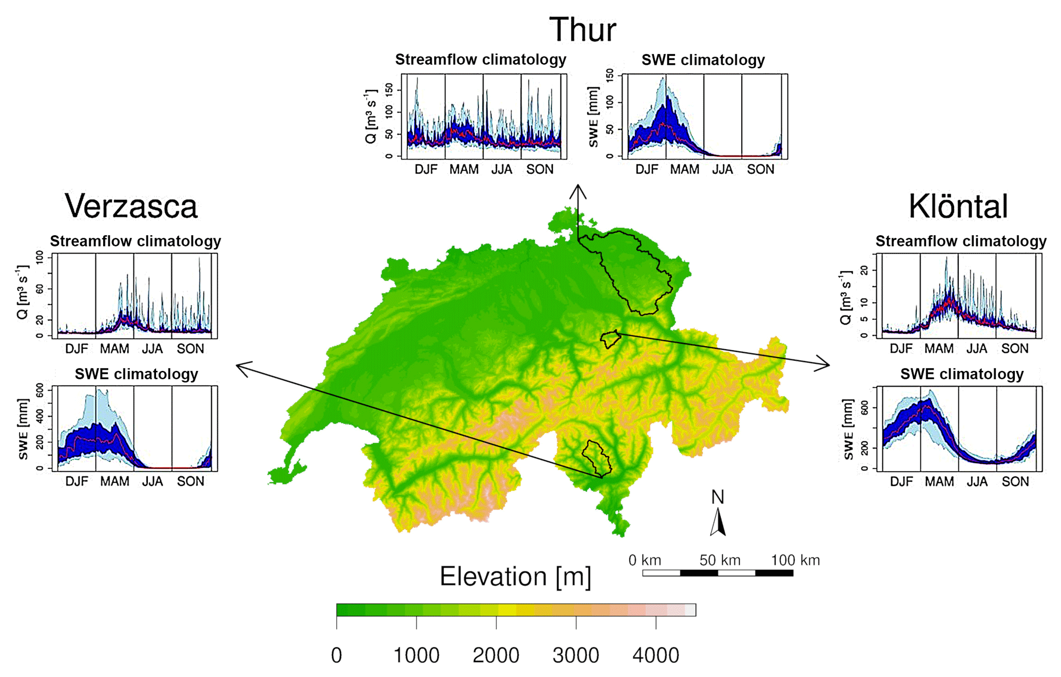
Figure 2Location and extent of the three selected catchments and their corresponding streamflow and SWE climatology. The Verzasca catchment in the south, the Klöntal catchment in the centre, and the Thur catchment in the north-east.
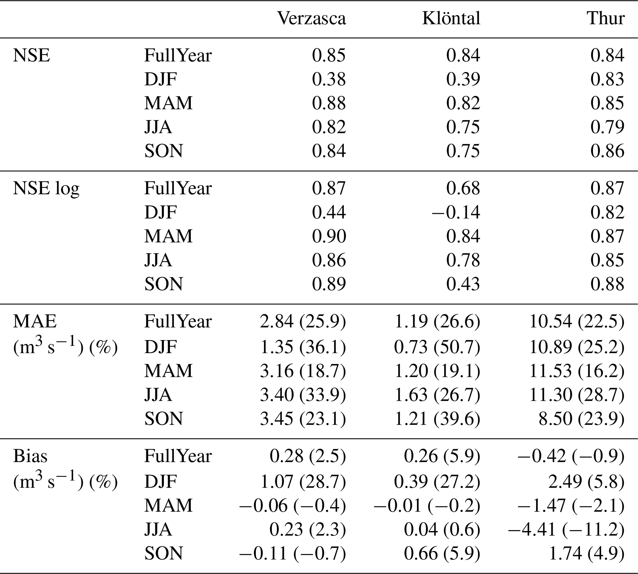
Table 2Verification of the reference simulation with corresponding observations for the Verzasca catchment, the Klöntal catchment, and the Thur catchment. In each catchment the NSE, the NSE log, the bias, and the mean absolute error are shown. The verification is done for the full simulation period (FullYear: 1994–2014) and the individual seasons within the full period (DJF, MAM, JJA, SON). A perfect simulation would have NSE=1, and positive values of NSE indicated better skill than the reference climatology.
4.1 Performance of the reference simulation
The reference simulation is analysed over the full 20-year period of the reforecasts. The verification of the reference simulation against observations, summarized in Table 2, generally shows high agreement of the simulation with the corresponding observations.
The NSE coefficient for the entire analysis period (FullYear) exhibits values above 0.84 for all catchments. Best performance can be observed in spring and lowest performance in winter when low flows dominate. The logarithmic form of the NSE (NSE log) shows a similar picture with better performance in the Thur catchment. Some difficulties occur in DJF in the Verzasca catchment and in DJF and SON in the Klöntal catchment. In the Verzasca and the Klöntal catchment the MAE and the absolute bias are constant over the course of the year except in winter. But compared to the mean annual flows of the specific catchments largest relative biases are observed during DJF. The Thur catchment exhibits smallest relative biases except in JJA when low flows occur because of the absence of snow in this catchment. Various applications do not focus on low flows but rather on flow volumes, e.g. hydropower operations are more interested in forecasts about the total upcoming flow volume to adapt and optimize their production. Therefore, we here focus on the standard Nash–Sutcliffe coefficient instead of the logarithmic form thereof.
We hereafter verify streamflow predictions against the reference simulation to focus on analysing the effect of the different meteorological input forecasts. This allows us to solely assess the effect of the pre-processing on the hydrological predictions by suppressing the hydrological errors themselves and is often done to evaluate operational forecasting systems (Alfieri et al., 2014), to assess the contributions of uncertainty on the hydrological forecasts (Voisin et al., 2011), or for a comparison of the skill of different forecasting systems (Pappenberger et al., 2015). Such an evaluation against a reference simulation also minimizes the influence of the deficits of the hydrological model under low-flow conditions on the verification analysis as found for the reference simulation described above. However, the effect of pre-processing on the performance if real observations are used for the verification reveals interesting aspects of the deficits of the hydrological simulations and will be discussed in Sect. 5.
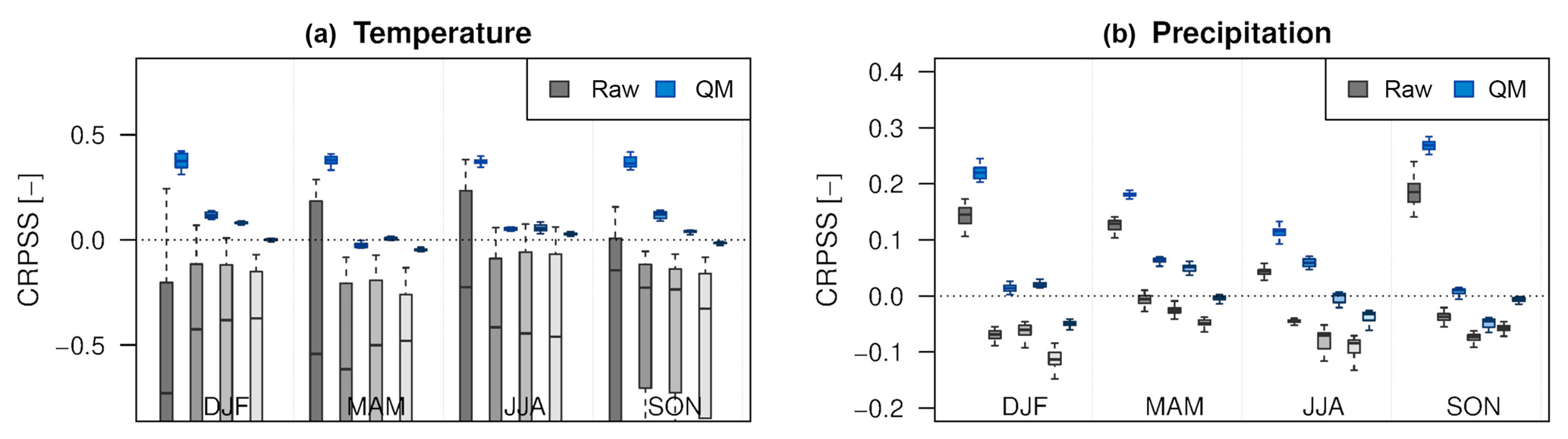
Figure 3Overview of the CRPSS for weekly mean temperatures (a) and weekly precipitation sums (b) in 1994–2014 reforecasts grouped by season (DJF, MAM, JJA and SON) for all grid points within the Verzasca catchment. The shading of the boxes denotes lead time, where week 1 corresponds to day 5–11, week 2 to days 12–18 and so on. Grey shading for raw forecast and blue shading for pre-processed reforecasts. An individual box shows the distribution of the CRPSS for all grid points within the catchment averaged over all 13 reforecast initialization dates within one season. The boxes depict the interquartile range, the mean is indicated by the horizontal line and the whiskers span the length of 1.5× standard deviation of the data. A perfect forecast has CRPSS=1, and positive values indicate better skill than the reference climatology.
4.2 Skill of the meteorological input
The raw and bias-corrected temperature and precipitation reforecasts used to drive the hydrological predictions are verified against the gridded observations in the Verzasca domain. In Fig. 3, the CRPSS for the raw and bias-corrected temperature and precipitation reforecasts is shown. Raw temperature reforecasts mainly exhibit negative CRPSS values, indicating essentially no skill compared to climatology. After bias correction using the quantile mapping technique the reforecasts exhibit positive CRPSS up to 18–24 lead days in all seasons but spring (MAM). Raw precipitation reforecasts exhibit positive skill for lead days 5–11 in all seasons and negative CRPSS for longer lead times. After bias correction the skill is higher, with a positive CRPSS of up to 3 weeks in MAM. In JJA the positive skill is only observed for a 2-week lead time and in SON and DJF for the first week only. Similar results are obtained for the Klöntal and the Thur catchment (not shown).
4.3 Streamflow prediction performance
4.3.1 Prediction performance
The performance of the reforecasts is analysed for all available reforecast dates within the period 1994–2014. In Fig. 4 the resulting scores (NSE, Bias, CRPSS, and the spread–error ratio) for all three catchments are presented, indicating the skill of the prediction system against the reference simulation, i.e. the expected performance of the system for any date throughout the year.
For the Verzasca catchment, the skill in terms of the NSE from the ESPs suddenly drops after the initialization of the forecasts, whereas the prediction system using meteorological reforecasts provides positive NSE up to 7 days. Pre-processing of precipitation generally even lowers the NSE, indicating positive skill only for 5 lead days. Pre-processing of temperature does enhance the skill with positive NSE up to a 13-day lead time. If both variables (precipitation and temperature) are pre-processed the positive effect of the temperature pre-processing on NSE is diminished by the negative effect of precipitation pre-processing.
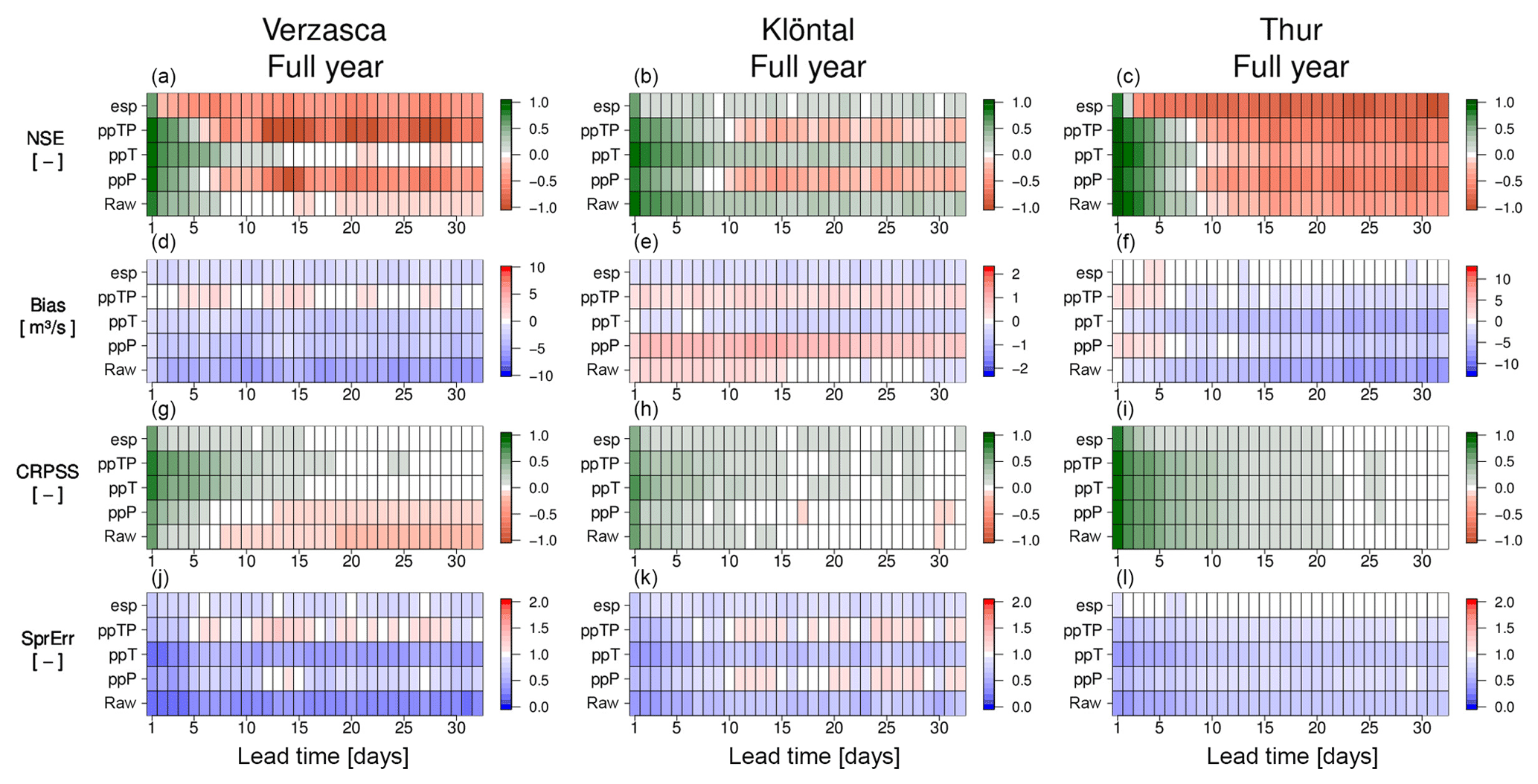
Figure 4Verification of the streamflow forecasts for the Verzasca (a), Klöntal (b), and Thur (c) catchments considering all forecasts within the reforecast period. The NSE coefficient in the upper most panel, the mean bias (Bias) in the second, the CRPSS in the third, and the spread-error relationship (SprErr) in the lowest panel. For each score the five different set-ups are shown. The first row corresponds to the ESP approach (esp), the second row to the reforecasts using both pre-processed temperature and precipitation (ppTP), the third row to the pre-processed temperature-only (ppT), the fourth row to the pre-processed precipitation-only (ppP), and the fifth row to the reforecasts using the raw meteorological input reforecasts (raw). The NSE and the CRPSS span from −infinity to 1, with a perfect score being 1; a bias of 0 indicates no forecast error, with negative values indicating underestimation and positive values indicating overestimation of the flow; reliable forecasts exhibit a SprErr of 1, lower values indicate overconfidence, and greater values indicate overdispersion.
The negative biases of the ESP approach indicate an underestimation of the streamflows for all lead times in the Verzasca catchment. Raw forecasts show even stronger underestimation. After pre-processing either precipitation or temperature, this underestimation is lower and reaches similar biases to the ESPs. If both parameters are pre-processed the biases are close to 0 or slightly positive, indicating that the streamflows are neither underestimated nor overestimated.
The overall performance characterized by the CRPSS indicates positive skill for the ESPs up to 15 days lead time for the Verzasca, but the skill drops quickly after the initialization of the forecasts as in the NSE. Raw forecasts only show a positive CRPSS for the first 5 lead days. Pre-processing of precipitation increases the CRPSS at short lead times. Temperature pre-processing enhances the skill at early lead times and in addition elongates positive skill up to 15 days lead time. This is even more pronounced if both variables are pre-processed.
The spread–error ratio of the ESPs is below 1 for all lead times, indicating overconfidence. For the NWP-Hydro-chain the overconfidence is even higher for raw and temperature-only pre-processed (ppT) reforecasts. Pre-processed precipitation (ppP) reforecasts can partly correct the overconfidence of the streamflow reforecasts and if both variables are pre-processed (ppTP), the spread–error ratio indicates reliable forecasts.
These skill signatures are similar in the other two catchments analysed in this study (Fig. 4), although not in an absolute sense. In the small, semi-glaciated Klöntal catchment the absolute skill generally is higher, and the skill of the predictions extends to longer lead times. In particular the raw and temperature-only pre-processed reforecasts (ppT) show positive skill in terms of the NSE throughout all lead times. In the Thur catchment the skill of the raw reforecasts outperforms the ESPs as well, but in contrast to both other catchments, the effect of pre-processing is negligibly small.
4.3.2 Seasonal variations in skill
The prediction skill of the different approaches does not only vary across catchments, but also across seasons. In Fig. 5 the performance in the Verzasca catchment for the four seasons DJF, MAM, JJA, and SON is shown. The general characteristics are similar to those observed for the entire year; i.e. the ESP-based predictions exhibit a sudden drop in the NSE after initialization and most benefits (positive skill to longer lead times) are obtained if temperature-only is pre-processed (ppT). In DJF and MAM this skilful horizon is extended by ppT, from 5 (3) days to up to 16 (9) days in MAM (DJF), and the bias is reduced.
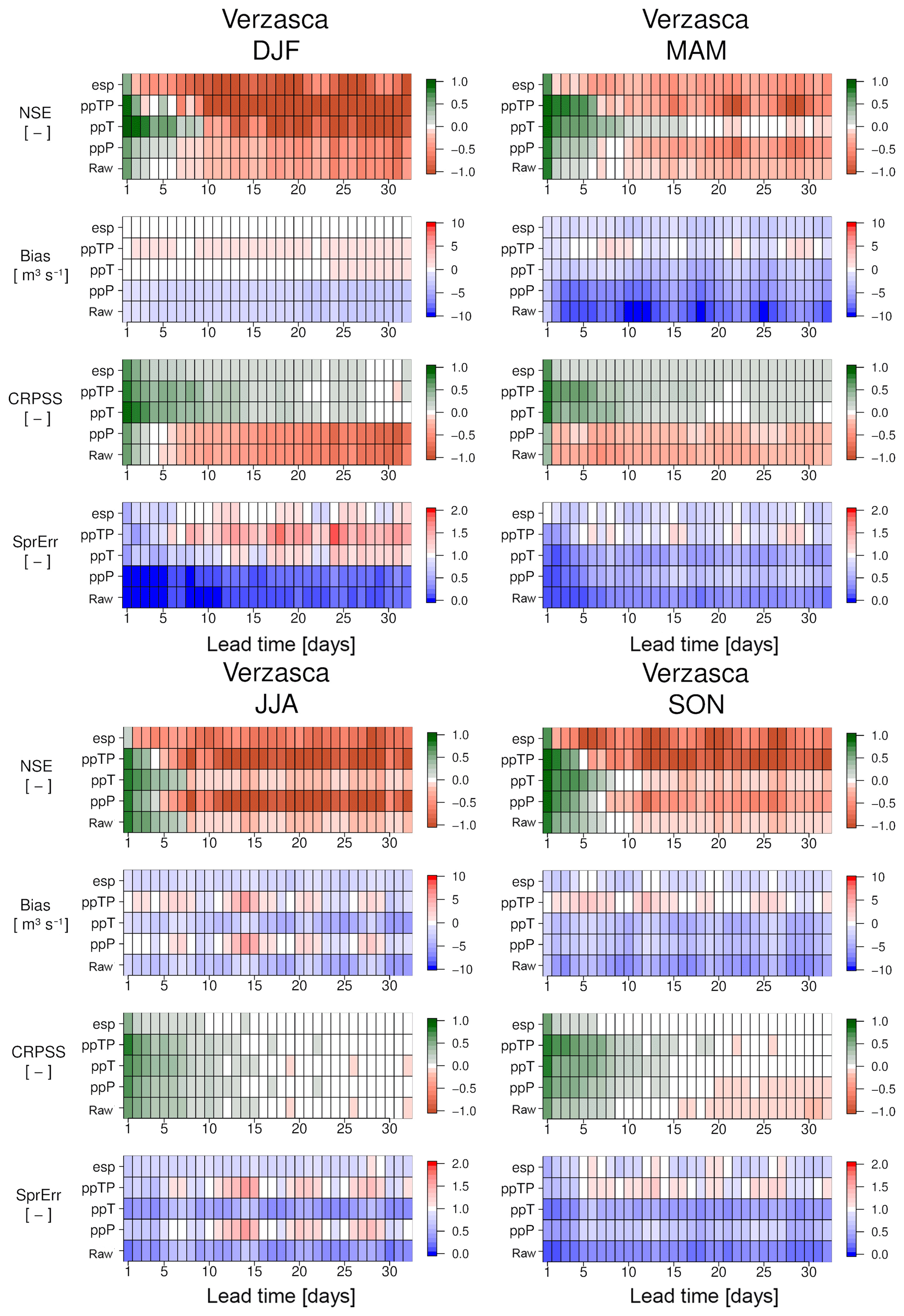
Figure 5Same as Fig. 4 but seasonally aggregated (DJF, MAM, JJA, and SON) for the Verzasca catchment.
The overall performance (CRPSS) for the ESPs is better than the reference climatology for all lead times in MAM and clearly outperforms the raw reforecasts and precipitation-only pre-processed reforecasts (ppP) in MAM and DJF. For the temperature-only pre-processed reforecasts (ppT) and if both variables are pre-processed (ppTP), the predictions in these seasons (DJF and MAM) outperform the ESP forecasts for lead times up to 12 to 15 days and are equal for longer lead times. In JJA (and SON, not shown) the ESPs only exhibit a positive CRPSS up to 5 and 9 days, whereas the raw reforecasts (i.e. without any pre-processing) indicate positive skill up to lead times of 10 and up to 15 days. However, in contrast to DJF and MAM, the influence of the pre-processing on the performance is negligible in JJA. Furthermore, in JJA the bias and the spread–error ratio are only better if the pre-processing includes precipitation.
The seasonal variation in performance holds true as well for the other catchments, i.e. reforecasts initiated in winter and spring show highest benefits over the reference climatology. In contrast to the Verzasca catchment, the raw and precipitation only pre-processed reforecasts show higher streamflows than the reference climatology in MAM and the raw and temperature pre-processed reforecast show a positive NSE up to 30 lead time days (Fig. 6, left).
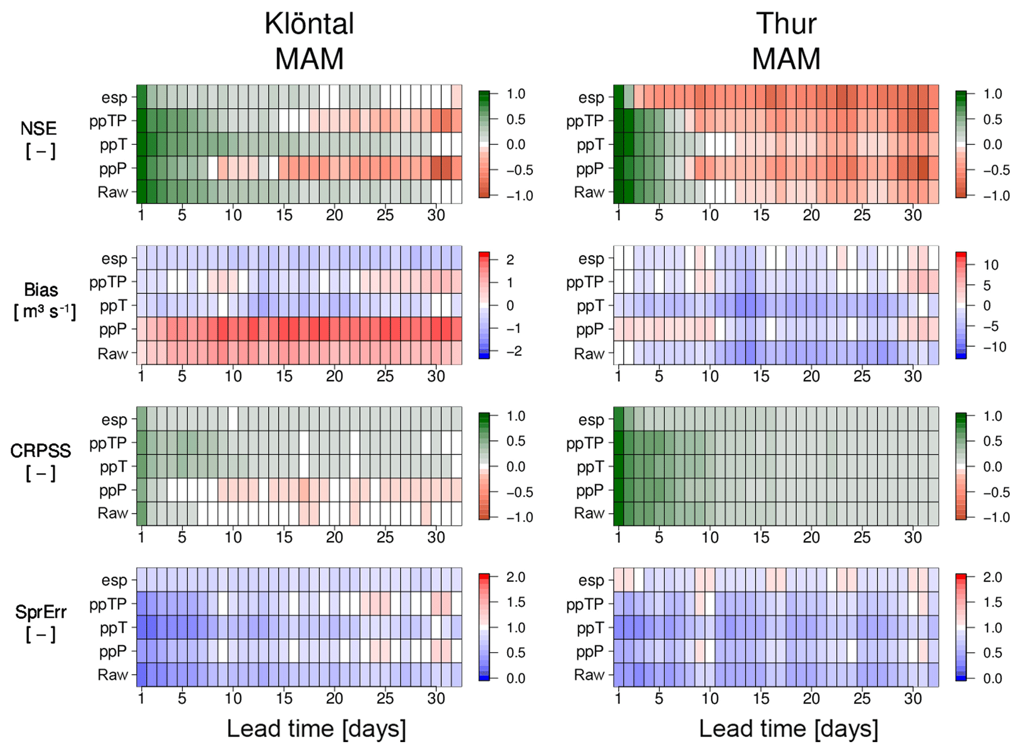
Less seasonal variation is observed in the Thur catchment although the general signatures are evident as well. In MAM (Fig. 6, right) all methods perform better than the reference simulation (positive CRPSS) over the full forecast range. Generally worst performance is found for the ESP. The effect of the pre-preprocessing is limited and can mainly be noticed if precipitation is pre-processed, resulting in smaller biases and a spread-to-error ratio closer to 1, indicating a reduction in overconfidence.

Figure 7Rank histograms for all four configurations (raw, ppP, ppT, ppTP) and the ESPs for the full analysis period (Full year) and MAM in the Verzasca catchment. The basic principle in the rank histograms the assumption that the ensemble members determine bins in which the corresponding observation can be ranked. For a reliable forecast, the observations are equally distributed across all different bins resulting in a uniform shape of the rank histograms. If for example the frequency in the lowest (rank 0) and the highest bin (rank 6) is much higher, the observation tends to be more frequently either higher than all ensemble members or lower than all ensemble members but less often in between the ensemble members. This specific U-shape indicates that the forecast spread is too narrow and thus the forecasts generally overconfident. In contrast, if the observations tend to be more often in between the ensemble members (e.g. rank 2 and 3), the rank histogram exhibit a convex shape and thus the forecast spread is too large indicating overdispersive forecasts.
4.3.3 Reliability of the ensembles
An additional important forecast characteristic is the reliability of the predictions, which cannot directly be deduced from the metrics shown above. Therefore, the rank histogram for the full period (Full year) and MAM reforecasts in the Verzasca catchment for all model configurations is shown in Fig. 7 to assess the reliability of the streamflow forecasts. As an example we focus on the rank histograms of the full period (Full year) and the MAM reforecasts, because of its representativeness for the seasonality of performance. In MAM, both versions, raw and precipitation-only pre-processed reforecasts, show an underestimation of the flows (negative bias) indicating that most reforecast members tend to be lower than the corresponding observations. The strong negative bias is reduced if temperature-only pre-processed reforecasts (ppT) are used. But still a U-shape is evident in the histograms that indicates overconfidence and thus confirms the conclusions from the spread–error ratio.
If both temperature and precipitation is pre-processed (ppTP) the resulting rank histograms become more uniform, in particular for longer lead times indicating a reduction of the overconfidence. But shorter lead times still exhibit some overconfidence. The rank histograms for the ESPs do provide more uniform rank histograms with a weak tendency of a negative bias. Although slight differences can be observed between different seasons, the main characteristics are similar for the full period.
The rank histograms for the Klöntal and Thur catchments (supplementary material) exhibit the same general behaviour regarding the reliability, but improvements by pre-processing are less pronounced for the Thur catchment and the rank histograms still indicate overconfidence even if both variables are pre-processed.
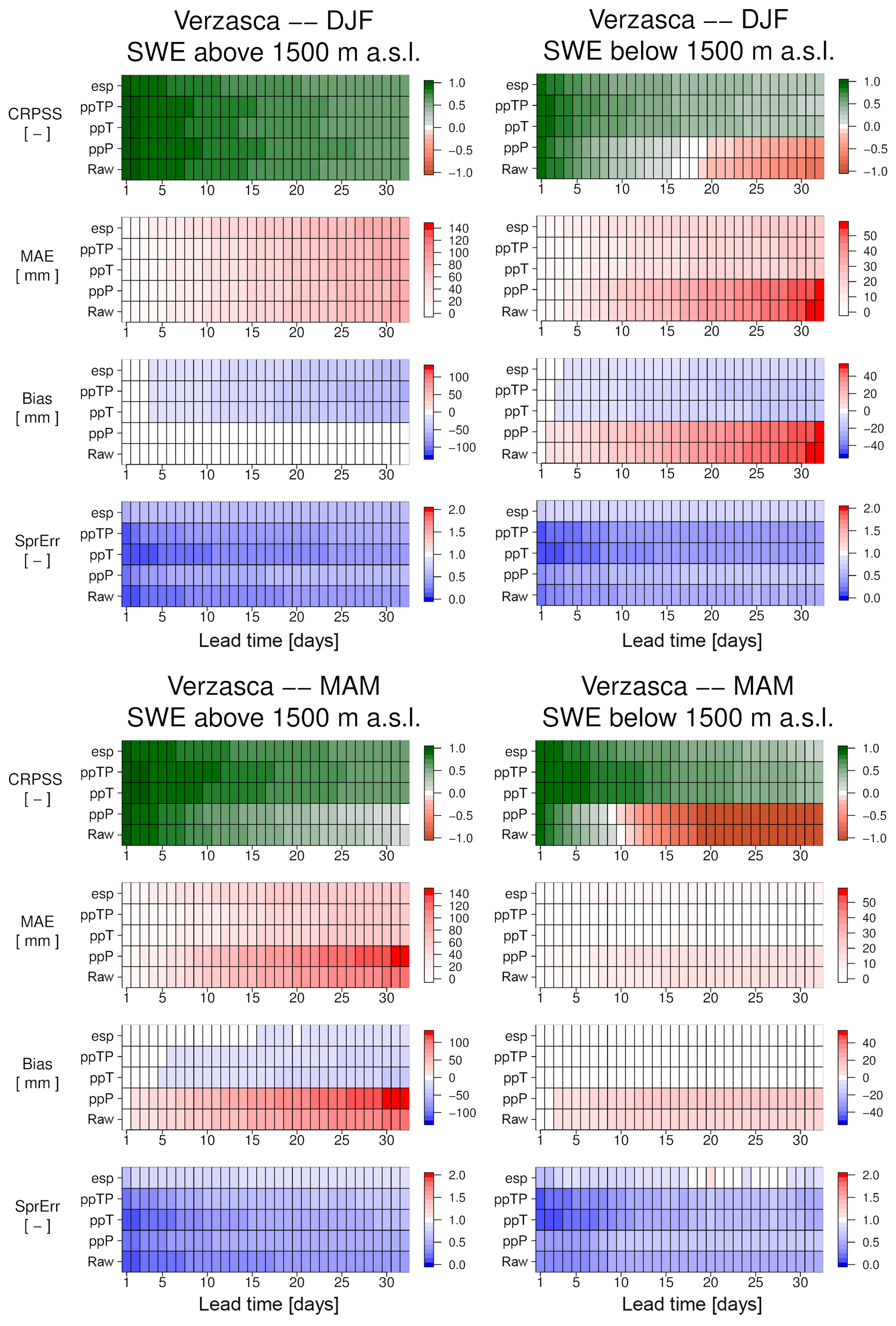
4.3.4 Snow water equivalent verification
To generate skilful streamflow predictions in mountainous catchments, the snow in the catchment is a crucial variable. Therefore, the SWE in the hydrological model is analysed according to different elevation regions. For the verification we analyse the SWE at elevations above and below 1500 m a.s.l. As in the verification of the streamflow reforecasts, the SWE is verified against the SWE of the reference simulation to replace the observations. A verification of modelled SWE against a consistent and homogenized climatology of gridded SWE based on station information is given by Jörg-Hess et al. (2014). They have shown that the modelled SWE exhibits errors that are of the same order as natural variability.
In MAM, raw and precipitation-only pre-processed (ppP) reforecasts highly overestimate the SWE in areas above 1500 m a.s.l. indicated by the MAE and the bias in Fig. 8. The predictive skill in terms of the CRPSS is lost after a 9-day lead time. In contrast, the reforecasts in DJF show stronger overestimation in areas below 1500 m a.s.l. and a total loss of predictive skill after a 15-day lead time in this area. The lowest biases and highest skill (in terms of the CRPSS) are evident for reforecasts with pre-processed temperature and precipitation (ppTP), followed by temperature-only pre-processed (ppT), both outperforming the ESPs.
For all versions of the meteorological reforecasts (raw and pre-processed) the resulting SWE reforecasts tend to be overconfident, with least overconfidence if precipitation-only is pre-processed according to the spread–error ratio. The ESPs exhibit less overconfidence for both seasons and regions and exhibit similar levels in terms of MAE and the bias and slightly less overall skill (CRPSS) compared to ppT and ppTP reforecast versions.
The rank histograms confirm the conclusion drawn above. Raw and precipitation-only pre-processed reforecasts (ppP) exhibit largest positive biases throughout all lead times. In case of temperature-only (ppT) and temperature and precipitation pre-processed reforecasts (ppTP) the rank histograms indicate overconfidence in the beginning which is reduced for longer lead times.
The SWE verification in the Klöntal catchment shows a similar behaviour with negative biases and largest MAE for the raw and precipitation-only pre-preprocessed (ppP) reforecasts. In contrast to the Verzasca catchment the CRPSS stays positive for all versions and for all lead times. A similar behaviour is observed in the Thur catchment with positive skill for all lead times but smaller negative biases (the corresponding figures for the Klöntal and the Thur catchment can be found in the Supplement).
For a proper evaluation of the effect of pre-processing on the hydrological streamflow predictions the following discussion considers the verification against the reference simulation. The meteorological input reforecasts highly benefit from the pre-processing procedure applied. The skill found for the pre-processed temperature and precipitation reforecast is comparable to the skill found in Monhart et al. (2018). In contrast to the present analysis, our earlier study used station-wise post-processing of the raw forecasts using the same set-up as in the present study. Similarly, different studies emphasize the benefit of pre-processing precipitation (Crochemore et al., 2016) and temperature forecasts (Lucatero et al., 2018a) at catchments at various spatial scales. The QM method used here is a popular pre-processing method for hydrometeorological ensemble forecasts (e.g. Kang et al., 2010; Lucatero et al., 2018b; Verkade et al., 2013) but does not come without limitations. In particular Zhao et al. (2017) point out the inability of QM to provide fully reliable ensembles for post-processing GCM precipitation. However, an extensive discussion of the reliability issue of the pre-processed meteorological input data used in this study can be found in Monhart et al. (2018). To summarize, it was found that the combination of the NWP model with QM indeed is able to provide reliable ensembles for lead times beyond 10 days but at shorter lead times the ensembles tend to be overconfident because the spread in the underlying NWP forecasts tends to be inappropriate what cannot be corrected using QM. An additional critical limitation of QM is the issue of variance inflation. Maraun (2013) emphasizes that the variance of the downscaled product strongly depends on the variance of the raw model grid box and QM does not introduce any small-scale variability. This is of particular importance for applications using local-scale information (such as distributed hydrological modelling) and if extremes are considered. In CH2018 (2018) these limitations of the QM method are highlighted for local climate change scenarios in Switzerland. In particular for convective precipitation events in summer the variance inflation issue can cause misinterpretation of data at the finer resolved scale. In the present study we are interested in the average streamflow throughout all season in the year for the upcoming 32 days and not in predicting extremes what reduces these implications, but still the spatial structure especially during convective situations in summer will likely be misrepresented and can influence the results. Different alternatives could be used depending on the specific application of the downscaled information, e.g. perfect prognosis approaches (Von Storch, 1999), the use of weather generators (e.g. Peleg et al., 2017) or in general stochastic methods (e.g. Volosciuk et al., 2017). However, such methods often require large computational resources. As the intention of this study is to pioneer the use of subseasonal hydrological predictions towards an operational use, we decided to use the QM technique despite its limitations. The results presented above and discussed in the following paragraphs legitimate our choice. Nevertheless, future studies should focus on the effect of variance inflation when QM is used to pre-process the predictions and alternative methods should be considered.
Our results show that subseasonal streamflow predictions in mountainous catchments can be skilful for the full 32-day lead time horizon in winter and spring. The traditional ESP approach clearly provides skilful predictions for all three catchments analysed in this study, in terms of the overall skill (CRPSS) and the reliability. This is in agreement with the findings from Arnal et al. (2018) comparing the skill of an ESP and a seasonal forecasting system across many regions in Europe. They found that the ESP approach can be outperformed mainly in the first month in terms of the CRPSS. Nevertheless, if scores evaluating the mean characteristics are considered (NSE and bias), we observe worse performance than suggested by the CRPSS. This indicates that the ESPs can capture the future evolution of the streamflow in a probabilistic sense. Furthermore, the substantial decrease in skill within the first days suggests that the ESPs are not able to capture the exact evolution, but can rather be used to estimate the general behaviour within the upcoming weeks. This is in agreement with the exponential decay in skill with increasing lead time found for ESP forecasts in UK catchments (Harrigan et al., 2018). If the NWPs are used to predict the streamflows, the skill can clearly be enhanced, but in most cases only if the driving meteorological predictions are pre-processed. This indicates that knowledge of the synoptic conditions plays an important role in enhancing the skill of the streamflow predictions at early lead times and that biases in these driving predictions need to be corrected prior to make these predictions useful. Furthermore, the improvements in performance of the streamflow predictions by pre-processing suggests that the gridded observational dataset provides a good baseline for this purpose, despite the difficulties involved in producing a gridded product based on a limited number of observational stations. In addition, the performance of the ESPs could potentially be enhanced if not all but only individual years are taken into account. A certain guidance based on a selection of years with similar initial conditions could be taken into account. Crochemore et al. (2017) have shown that seasonal prediction based on ESP can benefit from conditioning the forecasts on climatology. However, an evaluation of such an approach is beyond the scope of the present study.
The effect of pre-processing is even more pronounced for the SWE verification. In the NWP chain the SWE is highly overestimated if temperature is not pre-processed (raw and ppP). Hence, the hydrological model inherent downscaling of temperature using an adiabatic lapse rate leads to low skill in terms of CRPSS at longer lead times. Although temperature lapse rate corrections have been found to be important for reproducing streamflow simulation based on regional climate model outputs in mountainous snow- and glacial-dominated catchments (Butt and Bilal, 2011; Rahman et al., 2014), our study suggests that at least in a subseasonal forecasting context such corrections are not sufficient. Similarly, Tobin et al. (2011) have shown that for a flood forecasting framework constant lapse rate corrections, even if seasonally derived, are unable to capture the dynamics of temperature changes during an event. At lower elevations this effect is even more crucial because the SWE is smaller and temperature biases accelerate melting processes in the model. If temperature pre-processing is included, these large errors can be avoided, and the skill of the SWE predictions is substantially increased. This effect underlines the importance of pre-processing the subseasonal forecast in snow-dominated catchments. The importance of the SWE initial conditions for subseasonal forecasts has been shown by Jörg-Hess et al. (2015a). They conclude that a better representation of snowmelt process by improved states of the snow storage can greatly improve the predictions of streamflow volumes. The influence of initial conditions of SWE on seasonal streamflow predictions in the US is shown by Wood et al. (2016) in an idealized experiment. Furthermore, they stress that limited skill in seasonal meteorological predictions can be amplified in streamflow prediction skill. Our study suggests that an additional pre-processing of the meteorological forecasts is necessary to maintain the benefit of the initial conditions and confirms the findings of amplified skill in the streamflow predictions if the forecasts exhibit some skill. Otherwise, low skill in performance of the (raw) forecasts and the loss in skill to predict the SWE over longer lead times directly translates into low skill of the streamflow forecasts.
The comparison of the performance in the three different catchments analysed gives further insight into the predictability of streamflows in alpine catchments and strengthens the picture drawn above which shows the importance of the complex interactions between precipitation, temperature, and SWE at the subseasonal forecast timescale. In the Thur catchment, the largest catchment in the analysis, which is mainly precipitation dominated, the difference in skill between the ESPs and the NWP-based prediction is smallest. Similarly, the differences between raw and pre-processed experiments are marginal. Only in spring, if precipitation is pre-processed (ppP and ppTP), can a small improvement in the CRPSS be observed at early lead times coinciding with the lead times where pre-processed precipitations still exhibit skill. Hence the initial conditions of the model and skilful precipitation predictions at early lead times determine to a large degree the skill of the reforecasts, and the negligible snow-covered area within the catchment does marginally affect the performance of the runoff predictions. In the Thur catchment two additional subcatchments in the upper Thur catchment (at runoff stations Halden and Murg) have been verified to identify the influence of hilliness and catchment size on the forecast performance. Although the sizes of the Murg (212 km2) and the Halden catchment (1085 km2) vary significantly, the hilliness in both is comparable, while the lower part of the Thur catchment (station Andelfingen, 1696 km2) is a typical lowland region. For all three stations the skill is very similar (Fig. S4 in the Supplement) and pre-processing does not vary either. This suggests that neither hilliness nor catchment size significantly influences the performance of the forecast. In the snow-dominated and partially glaciated Klöntal catchment, the smallest catchment in this analysis, the high skill in terms of the NSE indicates a good performance of the ensemble mean, but in terms of the overall skill (CRPSS) the NWPs are only skilful if temperature pre-processing is considered. This superiority in the mean is most likely the effect of melting processes. On the other hand, the Verzasca catchment is snow dominated in elevated regions but rain dominated at lower elevations due to its large gradient of elevations. Therefore, snowmelt processes tend to occur more often and are more diverse due to the higher-elevation gradient within the catchment. The NSE does indicate skill up to a 13-day lead time for the temperature-only pre-processed forecast (ppT), but precipitation pre-processing even lowers the skill despite an increase in skill of the corresponding precipitation inputs. This counterintuitive behaviour of lowering the skill (in terms of NSE) in the streamflow prediction despite the use of improved precipitation inputs underlines that for a profound assessment of the skill of ensemble forecasts, verification metrics focusing on mean flows can be insufficient and misleading.
The combination of pre-processed subseasonal meteorological prediction with hydrological simulations can outperform a traditional ESP approach in small to medium-sized alpine catchment. Especially in snow-dominated and (semi-)glaciated catchments such a prediction chain brings large benefits in the forecast performance. But temperature (and precipitation) from the NWP model needs to be pre-processed prior to be used in hydrological models to achieve better performance than an ESP approach. In precipitation-dominated catchments the pre-processing only shows a marginal improvement in skill, but the NWP chain clearly outperforms ESPs. Hence, such systems can be of interest for application when accurate and reliable runoff predictions are desired, especially in snow-dominated catchments. Furthermore, Frei et al. (2018) have shown that a general decrease in snowfall is expected in future climate change scenarios, while at higher elevation the signal shows a slight increase in heavy snowfall events, due to a shift of climatological cold areas into a temperature interval which favours higher snowfall intensities in combination with a general increase in winter precipitation. Especially regarding future scenarios which expect an increase in hydro power production due to melt water in the period from October to April (Weingartner et al., 2013) such systems might become a valuable tool for optimizing hydropower production in mountainous areas. Future work should include statistical post-processing techniques (of the hydrological output) to correct the errors and biases of the hydrological simulation and to account for additional uncertainty induced by the hydrological model in the ensemble.
The discussion above focused on the effect of pre-processing hydrometeorological predictions and therefore only the verification against the reference simulation was considered and hydrological model errors are thus excluded from the analysis. However, to estimate the real-world performance, the hydrological model errors need to be taken into account. To do so we verified the streamflows of the reference simulation of the PREVAH model against observations. The evaluation presented in Sect. 4.1 revealed the good performance of the hydrological model with NSE above 0.8 in most seasons. The largest difficulties are observed in seasons with low-flow conditions (in DJF in the Verzasca, and in SON and DJF in the Klöntal catchment). This is particularly evident in the logarithmic version of the NSE, in which flood peaks are flattened to better assess the performance under low-flow conditions: the difficulties of the model remain. These deficits of the hydrological model need to be considered in the verification of the predictions and are the reason for verifying the reforecasts against the pseudo observations from the reference simulation. Otherwise, if the predictions are verified against real streamflow observations, the hydrological model deficiencies dominate the skill characteristics of the predictions and possibly impede the identification of the effect of pre-processing. An example of such a deficiency is the uncertainty resulting from the hydrological modelling that results in stronger overconfidence especially at short lead times when the hydrological model uncertainty may be the dominant source of uncertainty as discussed for example in Bennett et al. (2014). To illustrate this for the prediction used in this study, the verification was repeated with the real runoff observations. The skill in most seasons (MAM, JJA, SON) exhibits the same behaviour with high skill at early lead times and decreasing skill at longer lead times, and generally higher overconfidence at short lead times is observed, which confirms the findings by Bennett et al. (2014). But during low-flow conditions (in DJF in the Verzasca catchment and in DJF and SON in the Klöntal catchment), strong negative peaks in skill (in terms of the CRPSS) are present at short lead times, with increasing skill at longer lead times (supplementary material). The corresponding input data revealed that this behaviour can be associated with predicted snowmelt events that coincide with observed “no melt” events. During such events, all members of the experiments including pre-processed temperatures (ppT and ppTP) overestimate the observed runoff peak. The comparison of the meteorological input data from the reforecast with data from an observational station shows an overestimation in both temperature and precipitation. The temperature observations for this event were clearly below freezing, whereas the raw forecast data are close to 0 ∘C, and the pre-processed temperature is positive. Hence, the melt-affected area is too large, leading to an overestimation of the runoff contribution. In addition, overestimated precipitation will further contribute to runoff, and less deposition of solid precipitation will occur. Similarly, the reference simulation does overestimate the runoff peak because of an overestimation of the temperature in the gridded data used to run the hydrological model. It is known that gridded observations do inherit errors due to interpolation (Freudiger et al., 2016) and do have difficulties in resolving small-scale features, such as cold pools in Alpine valleys (Frei, 2014). This can partly explain this behaviour. Another potential explanation is an insufficient formulation of the discrimination between rain and snow in the hydrological model. In the version of PREVAH used for this study, the formulation follows a threshold-based method in combination with a linear range as described in Zappa et al. (2003). This linear transition range is set between the threshold values −1.5 and +1.5 ∘C as determined by the hydrological calibration. The threshold itself and the corresponding linear range highly depend on the hydroclimatic characteristics and thus can strongly vary in space (Liu et al., 2018). It has been shown that more sophisticated approaches using logistic regression for characterizing this range can provide better results (Frei, 2016). In principle such an approach could be included in the hydrological model, but such an implementation is out of the scope of this analysis. Alternatively, it has been shown that such errors of the hydrological model can be corrected by additionally post-processing the hydrological output using neuronal networks or logistic regressions (e.g. Bogner et al., 2016; Sharma et al., 2018).
Recent advances in subseasonal meteorological ensemble models makes it feasible to develop hydrometeorological prediction systems driven by such NWP forecasts. We developed an end-to-end hydrometeorological prediction system driven with reforecasts from the subseasonal prediction system from the ECMWF. A pre-processing procedure based on QM is used to bias correct and downscale the meteorological predictions prior to the hydrological model. The performance of the resulting streamflow forecasts is assessed for three small- to medium-sized alpine catchments using various verification metrics to assess different attributes of the reforecasts. Our study demonstrates the potential of ensemble streamflow predictions in small mountainous catchments. Moreover, the benefits of combining NWPs and hydrological models has been shown. The analysis indicates the need for pre-processing of the driving meteorological prediction especially in small snow-dominated catchments in alpine regions.
Decent skill of traditional ESPs compared to climatological reference can extend up to the entire 32 days. The NWP approach outperforms the ESPs in all catchments and most seasons in particular at short lead times up to about day 5. In snow-dominated catchments, an additional pre-processing step of both temperature and precipitation is crucial to further enhance the skill and the reliability of the forecasts. While pre-processing precipitation-only is not sufficient to enhance the forecast performance, it is crucial in the combination with temperature preprocessing to improve the forecast reliability. Again, it is noted here that the verification is done against the reference simulation as replacement of real observations. Hence, the performance cannot directly be interpreted as the prediction performance in an absolute sense, because in our approach the deficits of the hydrological model are not fully taken into account. However, the relative benefits of using NWP output as forcing for the hydrological simulations and the improvements after pre-processing is expected to hold true as well with real observations.
The benefits of the NWP approach and the pre-processing step is most pronounced in winter and spring when snowmelt processes dominate. This demonstrates the importance of snow for the predictability of streamflows at the subseasonal timescale. Hence the deficits in the hydrological model with respect to snow-related processes (in particular the distinction between solid and liquid precipitation) should receive further attention to enhance the forecast performance. Alternatively, post-processing techniques applied to the streamflow forecasts can be applied to correct such hydrological model deficits. This would allow assessment of the skill of the forecasts with respect to real observations and can potentially further increase the performance of the forecasts. Hence, if post-processing techniques are able to account for the deficits of the reference simulation, the combination of both pre- and post-processing could provide skilful lead streamflow predictions in snow- and glacial-dominated catchments in mountainous terrain at the subseasonal forecast horizon.
Furthermore, technical improvements of the NWP models related to the ensemble size, frequency of issuing reforecasts, and improvements in the representation of physical processes can be expected to have a positive effect on the resulting streamflow performance. In our set-up we use a rather simple statistical bias correction technique to pre-process the hydrometeorological prediction. More sophisticated pre-processing techniques could be applied to analyse their capability to enhance the streamflow performance. Since ensemble hydrometeorological predictions are of interest for specific applications the forecasts should further be analysed according to their economic value, for example, to optimize the revenues of existing hydropower plants in alpine regions or for early better preparedness of hydrological droughts.
ECMWF forecast data are accessible through the MARS archive: http://apps.ecmwf.int/archive-catalogue/ (last access: 1 August 2018); observation records used in this study are available from the following website: https://gate.meteoswiss.ch/idaweb/more.do (SwissMetNet, last access: 1 August 2018). Streamflow series and catchment boundaries are provided by the Swiss Federal Office for the Environment (FOEN).
The supplement related to this article is available online at: https://doi.org/10.5194/hess-23-493-2019-supplement.
To specify the authors' contributions, we use the CRediT taxonomy defining scientific roles. The definition of these roles can be found at https://casrai.org/credit/ (last access: 23 January 2019). SM performed the following roles: conceptualization, methodology, software, validation, formal analysis, visualization, and writing the original draft. MZ performed the following roles: conceptualization, methodology, writing, review and editing, funding acquisition, and project administration. CSp performed the following roles: conceptualization, methodology, writing, review and editing. CSc performed the following roles: conceptualization, methodology, writing, review and editing, and supervision. KB performed the following roles: conceptualization, methodology, writing, review and editing.
The authors declare that they have no conflict of interest.
Konrad Bogner's contribution is part of the Swiss Competence Centre for
Energy Research-Supply of Electricity (SCCER-SoE) and is funded by the
Commission for Technology and Innovation (CTI). Samuel Monhart's contribution
is financed by the Swiss National Science Foundation (SNSF) and was carried
out within the framework of National Research Programme “Energy Turnaround”
(NRP 70, grant 407040153929). The authors want to thank the three anonymous
reviewers for their insightful comments on the original
manuscript.
Edited by: Alexander
Gelfan
Reviewed by: three anonymous referees
Addor, N. and Fischer, E. M.: The influence of natural variability and interpolation errors on bias characterization in RCM simulations, J. Geophys. Res.-Atmos., 120, 10180–10195, https://doi.org/10.1002/2014JD022824, 2015.
Addor, N., Rohrer, M., Furrer, R., and Seibert, J.: Propagation of biases in climate models from the synoptic to the regional scale: Implications for bias adjustment, J. Geophys. Res.-Atmos., 121, 2075–2089, https://doi.org/10.1002/2015JD024040, 2016.
Alfieri, L., Pappenberger, F., Wetterhall, F., Haiden, T., Richardson, D., and Salamon, P.: Evaluation of ensemble streamflow predictions in Europe, J. Hydrol., 517, 913–922, https://doi.org/10.1016/j.jhydrol.2014.06.035, 2014.
Anderson, J. L.: A method for producing and evaluating probabilistic forecasts from ensemble model integrations, J. Climate, 9, 1518–1530, https://doi.org/10.1175/1520-0442(1996)009<1518:AMFPAE>2.0.CO;2, 1996.
Arnal, L., Cloke, H. L., Stephens, E., Wetterhall, F., Prudhomme, C., Neumann, J., Krzeminski, B., and Pappenberger, F.: Skilful seasonal forecasts of streamflow over Europe?, Hydrol. Earth Syst. Sci., 22, 2057–2072, https://doi.org/10.5194/hess-22-2057-2018, 2018.
Bauer, P., Thorpe, A., and Brunet, G.: The quiet revolution of numerical weather prediction, Nature, 525, 47–55, https://doi.org/10.1038/nature14956, 2015.
Beerli, R., Wernli, H., and Grams, C. M.: Does the lower stratosphere provide predictability for month-ahead wind electricity generation in Europe?, Q. J. Roy. Meteor. Soc., 143, 3025–3036, https://doi.org/10.1002/qj.3158, 2017.
Begert, M. and Frei, C.: Long-term area-mean temperature series for Switzerland – Combining homogenized station data and high resolution grid data, Int. J. Climatol., 38, 2792–2807, https://doi.org/10.1002/joc.5460, 2018.
Bennett, J. C., Robertson, D. E., Lal, D., Wang, Q. J., Enever, D., Hapuarachchi, P., and Tuteja, N. K.: A System for Continuous Hydrological Ensemble Forecasting (SCHEF) to lead times of 9 days, J. Hydrol., 519, 2832–2846, https://doi.org/10.1016/j.jhydrol.2014.08.010, 2014.
Bogner, K., Liechti, K., and Zappa, M.: Post-processing of stream flows in Switzerland with an emphasis on low flows and floods, Water-SUI, 8, 115, https://doi.org/10.3390/w8040115, 2016.
Bogner, K., Liechti, K., Bernhard, L., Monhart, S., and Zappa, M.: Skill of Hydrological Extended Range Forecasts for Water Resources Management in Switzerland, Water Resour. Manag., 32, 969–984, https://doi.org/10.1007/s11269-017-1849-5, 2018.
Bohn, T. J., Sonessa, M. Y., and Lettenmaier, D. P.: Seasonal Hydrologic Forecasting: Do Multimodel Ensemble Averages Always Yield Improvements in Forecast Skill?, J. Hydrometeorol., 11, 1358–1372, https://doi.org/10.1175/2010JHM1267.1, 2010.
Brown, J. D., Demargne, J., Seo, D. J., and Liu, Y.: The Ensemble Verification System (EVS): A software tool for verifying ensemble forecasts of hydrometeorological and hydrologic variables at discrete locations, Environ. Model. Softw., 25, 854–872, https://doi.org/10.1016/j.envsoft.2010.01.009, 2010.
Butt, M. J. and Bilal, M.: Application of snowmelt runoff model for water resource management, Hydrol. Process., 25, 3735–3747, https://doi.org/10.1002/hyp.8099, 2011.
CH2018: CH2018 – Climate Scenarios for Switzerland, Technical Report, National Center for Climate Services, Zurich, Chapter 5.7., 98–101, available at: https://www.nccs.admin.ch/nccs/de/home/klimawandel-und-auswirkungen/schweizer-klimaszenarien/technical-report.html, last access: 1 December 2018.
Cloke, H. L. and Pappenberger, F.: Ensemble flood forecasting: A review, J. Hydrol., 375, 613–626, https://doi.org/10.1016/j.jhydrol.2009.06.005, 2009.
Crochemore, L., Ramos, M.-H., and Pappenberger, F.: Bias correcting precipitation forecasts to improve the skill of seasonal streamflow forecasts, Hydrol. Earth Syst. Sci., 20, 3601–3618, https://doi.org/10.5194/hess-20-3601-2016, 2016.
Crochemore, L., Ramos, M.-H., Pappenberger, F., and Perrin, C.: Seasonal streamflow forecasting by conditioning climatology with precipitation indices, Hydrol. Earth Syst. Sci., 21, 1573–1591, https://doi.org/10.5194/hess-21-1573-2017, 2017.
Davolio, S., Diomede, T., Marsigli, C., Miglietta, M. M., Montani, A., and Morgillo, A.: Comparing different meteorological ensemble approaches: hydrological predictions for a flood episode in Northern Italy, Adv. Sci. Res., 8, 33–37, https://doi.org/10.5194/asr-8-33-2012, 2012.
Day, G. N.: Extended Streamflow Forecasting Using NWSRFS, J. Water Resour. Plan. Manag., 111, 157–170, https://doi.org/10.1061/(ASCE)0733-9496(1985)111:2(157), 1985.
Demargne, J., Wu, L., Regonda, S. K., Brown, J. D., Lee, H., He, M., Seo, D. J., Hartman, R., Herr, H. D., Fresch, M., Schaake, J., and Zhu, Y.: The science of NOAA's operational hydrologic ensemble forecast service, B. Am. Meteorol. Soc., 95, 79–98, https://doi.org/10.1175/BAMS-D-12-00081.1, 2014.
Díez, E., Primo, C., García-Moya, J. A., Gutiérrez, J. M., and Orfila, B.: Statistical and dynamical downscaling of precipitation over Spain from DEMETER seasonal forecasts, Tellus A, 57, 409–423, https://doi.org/10.1111/j.1600-0870.2005.00130.x, 2005.
ECMWF, Part V: Ensemble Prediction System in IFS Documentation Cy40r1, ECMWF, Reading, England, 1–25, 2014.
Ferro, C. A. T.: Fair scores for ensemble forecasts, Q. J. Roy. Meteor. Soc., 140, 1917–1923, https://doi.org/10.1002/qj.2270, 2014.
Frei, C.: Interpolation of temperature in a mountainous region using nonlinear profiles and non-Euclidean distances, Int. J. Climatol., 34, 1585–1605, https://doi.org/10.1002/joc.3786, 2014.
Frei, P.: Snowfall in the Alps: Evaluation and Projections based on the EURO-CORDEX Regional Climate Models, Sci. Rep. Meteoswiss, 101, 122 pp., 2016.
Frei, P., Kotlarski, S., Liniger, M. A., and Schär, C.: Future snowfall in the Alps: projections based on the EURO-CORDEX regional climate models, The Cryosphere, 12, 1–24, https://doi.org/10.5194/tc-12-1-2018, 2018.
Freudiger, D., Frielingsdorf, B., Stahl, K., Steinbirch, A., Weiler, M., Griessinger, N., and Seibert, J.: The Potential of meteorological gridded datasets for hydrological modeling in alpine basins, Hydrol. Wasserbewirts., 60, 353–367, https://doi.org/10.5675/HyWa_2016,6_1, 2016.
Fundel, F., Jörg-Hess, S., and Zappa, M.: Monthly hydrometeorological ensemble prediction of streamflow droughts and corresponding drought indices, Hydrol. Earth Syst. Sci., 17, 395–407, https://doi.org/10.5194/hess-17-395-2013, 2013.
García-Morales, M. B. and Dubus, L.: Forecasting precipitation for hydroelectric power management: how to exploit GCM's seasonal ensemble forecasts, Int. J. Climatol., 27, 1691–1705, https://doi.org/10.1002/joc.1608, 2007.
Gurtz, J., Baltensweiler, A., and Lang, H.: Spatially distributed hydrotope-based modelling of evapotranspiration and runoff in mountainous basins, Hydrol. Process., 13, 2751–2768, 1999.
Hamill, T. M. and Colucci, S. J.: Verification of Eta – RSM Short-Range Ensemble Forecasts, Mon. Weather Rev., 125, 1312–1328, 1997.
Hao, Z., Singh, V. P., and Xia, Y.: Seasonal Drought Prediction: Advances, Challenges, and Future Prospects, Rev. Geophys., 56, 108–141, https://doi.org/10.1002/2016RG000549, 2018.
Harrigan, S., Prudhomme, C., Parry, S., Smith, K., and Tanguy, M.: Benchmarking ensemble streamflow prediction skill in the UK, Hydrol. Earth Syst. Sci., 22, 2023–2039, https://doi.org/10.5194/hess-22-2023-2018, 2018.
Hersbach, H.: Decomposition of the Continuous Ranked Probability Score for Ensemble Prediction Systems, Weather Forecast., 15, 559–570, 2000.
Hock, R.: Temperature index melt modelling in mountain areas, J. Hydrol., 282, 104–115, https://doi.org/10.1016/S0022-1694(03)00257-9, 2003.
Hopson, T. M.: Assessing the Ensemble Spread – Error Relationship, Mon. Weather Rev., 142, 1125–1142, https://doi.org/10.1175/MWR-D-12-00111.1, 2014.
Inman, R. H., Pedro, H. T. C., and Coimbra, C. F. M.: Solar forecasting methods for renewable energy integration, Prog. Energy Combust. Sci., 39, 535–576, https://doi.org/10.1016/j.pecs.2013.06.002, 2013.
Isotta, F. A., Frei, C., Weilguni, V., Perčec Tadić, M., Lassègues, P., Rudolf, B., Pavan, V., Cacciamani, C., Antolini, G., Ratto, S. M., Munari, M., Micheletti, S., Bonati, V., Lussana, C., Ronchi, C., Panettieri, E., Marigo, G., and Vertačnik, G.: The climate of daily precipitation in the Alps: Development and analysis of a high-resolution grid dataset from pan-Alpine rain-gauge data, Int. J. Climatol., 34, 1657–1675, https://doi.org/10.1002/joc.3794, 2014.
Jaun, S., Ahrens, B., Walser, A., Ewen, T., and Schär, C.: A probabilistic view on the August 2005 floods in the upper Rhine catchment, Nat. Hazards Earth Syst. Sci., 8, 281–291, https://doi.org/10.5194/nhess-8-281-2008, 2008.
Jolliffe, I. T. and Stephenson, D. B.: Forecast Verification, edited by: Jolliffe, I. T. and Stephenson, D. B., John Wiley & Sons, Ltd, Chichester, UK., 2012.
Jörg-Hess, S., Fundel, F., Jonas, T., and Zappa, M.: Homogenisation of a gridded snow water equivalent climatology for Alpine terrain: methodology and applications, The Cryosphere, 8, 471–485, https://doi.org/10.5194/tc-8-471-2014, 2014.
Jörg-Hess, S., Griessinger, N., and Zappa, M.: Probabilistic Forecasts of Snow Water Equivalent and Runoff in Mountainous Areas, J. Hydrometeorol., 16, 2169–2186, https://doi.org/10.1175/JHM-D-14-0193.1, 2015a.
Jörg-Hess, S., Kempf, S. B., Fundel, F., and Zappa, M.: The benefit of climatological and calibrated reforecast data for simulating hydrological droughts in Switzerland, Meteorol. Appl., 22, 444–458, https://doi.org/10.1002/met.1474, 2015b.
Kang, T., Kim, Y., and Hong, I.: Comparison of pre- and post-processors for ensemble streamflow prediction, Atmos. Sci. Lett., 159, 153–159, https://doi.org/10.1002/asl.276, 2010.
Krause, P., Boyle, D. P., and Bäse, F.: Comparison of different efficiency criteria for hydrological model assessment, Adv. Geosci., 5, 89–97, https://doi.org/10.5194/adgeo-5-89-2005, 2005.
Kumar, S., Dirmeyer, P. A., and Kinter, J. L.: Usefulness of ensemble forecasts from NCEP climate forecast system in sub-seasonal to intra-annual forecasting, Geophys. Res. Lett., 41, 3586–3593, https://doi.org/10.1002/2014GL059586, 2014.
Lavers, D., Luo, L., and Wood, E. F.: A multiple model assessment of seasonal climate forecast skill for applications, Geophys. Res. Lett., 36, L23711, https://doi.org/10.1029/2009GL041365, 2009.
Liechti, K., Panziera, L., Germann, U., and Zappa, M.: The potential of radar-based ensemble forecasts for flash-flood early warning in the southern Swiss Alps, Hydrol. Earth Syst. Sci., 17, 3853–3869, https://doi.org/10.5194/hess-17-3853-2013, 2013.
Liu, Y., Ren, G., Sun, X., and Li, X.: A new method to separate precipitation phases, Hydrol. Earth Syst. Sci. Discuss., https://doi.org/10.5194/hess-2018-307, 2018.
Lucatero, D., Madsen, H., Refsgaard, J. C., Kidmose, J., and Jensen, K. H.: On the skill of raw and post-processed ensemble seasonal meteorological forecasts in Denmark, Hydrol. Earth Syst. Sci., 22, 6591–6609, https://doi.org/10.5194/hess-22-6591-2018, 2018a.
Lucatero, D., Madsen, H., Refsgaard, J. C., Kidmose, J., and Jensen, K. H.: Seasonal streamflow forecasts in the Ahlergaarde catchment, Denmark: the effect of preprocessing and post-processing on skill and statistical consistency, Hydrol. Earth Syst. Sci., 22, 3601–3617, https://doi.org/10.5194/hess-22-3601-2018, 2018b.
Manzanas, R., Gutiérrez, J. M., Fernández, J., van Meijgaard, E., Calmanti, S., Magariño, M. E., Cofiño, A. S., and Herrera, S.: Dynamical and statistical downscaling of seasonal temperature forecasts in Europe: Added value for user applications, Clim. Serv., 9, 44–56, https://doi.org/10.1016/j.cliser.2017.06.004, 2018.
Maraun, D.: Bias Correction, Quantile Mapping, and Downscaling: Revisiting the Inflation Issue, J. Climate, 26, 2137–2143, https://doi.org/10.1175/JCLI-D-12-00821.1, 2013.
Marsigli, C., Montani, A., and Paccagnella, T.: A spiatial verification method applied to the evaluation of high-resolution ensemble forecasts, Meteorol. Appl., 15, 125–143, https://doi.org/10.1002/met.65, 2008.
Meißner, D., Klein, B., and Ionita, M.: Development of a monthly to seasonal forecast framework tailored to inland waterway transport in central Europe, Hydrol. Earth Syst. Sci., 21, 6401–6423, https://doi.org/10.5194/hess-21-6401-2017, 2017.
Melsen, L., Teuling, A., Torfs, P., Zappa, M., Mizukami, N., Clark, M., and Uijlenhoet, R.: Representation of spatial and temporal variability in large-domain hydrological models: case study for a mesoscale pre-Alpine basin, Hydrol. Earth Syst. Sci., 20, 2207–2226, https://doi.org/10.5194/hess-20-2207-2016, 2016.
Meteoswiss: Documentation of MeteoSwiss Grid-Data Products Daily Mean, Minimum and Maximum Temperature: TabsD, TminD, TmaxD, Meteoschweiz Kundend., available at: https://www.meteoswiss.admin.ch/home/services-and-publications/produkte.subpage.html/en/data/products/2014/raeumliche-daten-temperatur.html (last access: 1 August 2018), 2016a.
MeteoSwiss: Documentation of MeteoSwiss grid-data products: Daily precipitation (final analysis): RhiresD, Meteoschweiz Kundend., available at: http://www.meteoswiss.admin.ch/home/services-and-publications/produkte.subpage.html/en/data/products/2014/raeumliche-daten-niederschlag.html (last access: 1 August 2018), 2016b.
Monhart, S., Spirig, C., Bhend, J., Bogner, K., Schär, C., and Liniger, M. A.: Skill of Subseasonal Forecasts in Europe: Effect of Bias Correction and Downscaling Using Surface Observations, J. Geophys. Res.-Atmos., 123, 7999–8016, https://doi.org/10.1029/2017JD027923, 2018.
Montani, A., Marsigli, C., Nerozzi, F., Paccagnella, T., and Buizza, R.: Nonlinear Processes in Geophysics Performance of the ARPA-SMR limited-area ensemble prediction system?: two flood cases, Nonlinear Process. Geophys., 8, 387–399, https://doi.org/10.5194/npg-8-387-2001, 2001.
Montani, A., Marsigli, C., Nerozzi, F., Paccagnella, T., Tibaldi, S., and Buizza, R.: The Soverato flood in Southern Italy: performance of global and limited-area ensemble forecasts, Nonlinear Process. Geophys., 10, 261–274, 2003.
Montani, A., Cesari, D., Marsigli, C., and Paccagnella, T.: Seven years of activity in the field of mesoscale ensemble forecasting by the COSMO-LEPS system: Main achievements and open challenges, Tellus A, 63, 605–624, https://doi.org/10.1111/j.1600-0870.2010.00499.x, 2011.
Müller, W. A., Appenzeller, C., Doblas-Reyes, F. J., and Liniger, M. A.: A debiased ranked probability skill score to evaluate probabilistic ensemble forecasts with small ensemble sizes, J. Climate, 18, 1513–1523, https://doi.org/10.1175/JCLI3361.1, 2005.
Nash, E. and Sutcliffe, V.: River flow forecasting through conceptual models Part 1 – A discussion of preinciples, J. Hydrol., 10, 282–290, 1970.
Ohmura, A.: Physical Basis for the Temperature-Based Melt-Index Method, J. Appl. Meteorol., 40, 753–761, https://doi.org/10.1175/1520-0450(2001)040<0753:PBFTTB>2.0.CO;2, 2001.
Orth, R. and Seneviratne, S. I.: Predictability of soil moisture and streamflow on subseasonal timescales: A case study, J. Geophys. Res.-Atmos., 118, 10963–10979, https://doi.org/10.1002/jgrd.50846, 2013a.
Orth, R. and Seneviratne, S. I.: Propagation of soil moisture memory to streamflow and evapotranspiration in Europe, Hydrol. Earth Syst. Sci., 17, 3895–3911, https://doi.org/10.5194/hess-17-3895-2013, 2013b.
Orth, R., Staudinger, M., Seneviratne, S. I., Seibert, J., and Zappa, M.: Does model performance improve with complexity? A case study with three hydrological models, J. Hydrol., 523, 147–159, https://doi.org/10.1016/j.jhydrol.2015.01.044, 2015.
Pappenberger, F., Ramos, M. H., Cloke, H. L., Wetterhall, F., Alfieri, L., Bogner, K., Mueller, A., and Salamon, P.: How do I know if my forecasts are better? Using benchmarks in hydrological ensemble prediction, J. Hydrol., 522, 697–713, https://doi.org/10.1016/j.jhydrol.2015.01.024, 2015.
Peleg, N., Fatichi, S., Paschalis, A., Molnar, P., and Burlando, P.: An advanced stochastic weather generator for simulating 2-D high-resolution climate variables, J. Adv. Model. Earth Sy., 9, 1595–1627, https://doi.org/10.1002/2016MS000854, 2017.
Rahman, K., Etienne, C., Gago-Silva, A., Maringanti, C., Beniston, M., and Lehmann, A.: Streamflow response to regional climate model output in the mountainous watershed: a case study from the Swiss Alps, Environ. Earth Sci., 72, 4357–4369, https://doi.org/10.1007/s12665-014-3336-0, 2014.
Rahman, M. M., Lu, M., and Kyi, K. H.: Seasonality of hydrological model spin-up time: a case study using the Xinanjiang model, Hydrol. Earth Syst. Sci. Discuss., https://doi.org/10.5194/hess-2016-316, in review, 2016.
Robertson, A. W., Kumar, A., Peña, M., and Vitart, F.: Improving and Promoting Subseasonal to Seasonal Prediction, B. Am. Meteorol. Soc., 96, ES49–ES53, https://doi.org/10.1175/BAMS-D-14-00139.1, 2015.
Schaake, J. C., Hamill, T. M., Buizza, R., and Clark, M.: HEPEX: The hydrological ensemble prediction experiment, B. Am. Meteorol. Soc., 88, 1541–1547, https://doi.org/10.1175/BAMS-88-10-1541, 2007.
Schär, C., Vasilina, L., Pertziger, F., and Dirren, S.: Seasonal Runoff Forecasting Using Precipitation from Meteorological Data Assimilation Systems, J. Hydrometeorol., 5, 959–973, https://doi.org/10.1175/1525-7541(2004)005<0959:SRFUPF>2.0.CO;2, 2004.
Schattan, P., Zappa, M., Lischke, H., Bernhard, L., Thurig, E., and Diekkruger, B.: An approach for transient consideration of forest change in hydrological impact studies, IAHS-AISH Proc. Reports, 359, 311–319, 2013.
Seck, A., Welty, C., and Maxwell, R. M.: Spin-up behavior and effects of initial conditions for an integrated hydrologic model, Water Resour. Res., 51, 2188–2210, https://doi.org/10.1002/2014WR016371, 2015.
Sharma, S., Siddique, R., Reed, S., Ahnert, P., Mendoza, P., and Mejia, A.: Relative effects of statistical preprocessing and postprocessing on a regional hydrological ensemble prediction system, Hydrol. Earth Syst. Sci., 22, 1831–1849, https://doi.org/10.5194/hess-22-1831-2018, 2018.
Sinha, T. and Sankarasubramanian, A.: Role of climate forecasts and initial conditions in developing streamflow and soil moisture forecasts in a rainfall-runoff regime, Hydrol. Earth Syst. Sci., 17, 721–733, https://doi.org/10.5194/hess-17-721-2013, 2013.
Speich, M. J. R., Bernhard, L., Teuling, A. J., and Zappa, M.: Application of bivariate mapping for hydrological classification and analysis of temporal change and scale effects in Switzerland, J. Hydrol., 523, 804–821, https://doi.org/10.1016/j.jhydrol.2015.01.086, 2015.
Von Storch, H.: On the use of “inflation” in statistical downscaling, J. Climate, 12, 3505–3506, https://doi.org/10.1175/1520-0442(1999)012<3505:OTUOII>2.0.CO;2, 1999.
Talagrand, O., Vautard, R., and Strauss, B.: Evaluation of probabilistic prediction systems, in Proceedings of a Workshop held at ECMWF on Predictability, 20–22 October 1997, Reading, UK, European Center for Medium-Range Weather Forecasts, 1–25, 1997.
Thirel, G., Martin, E., Mahfouf, J.-F., Massart, S., Ricci, S., Regimbeau, F., and Habets, F.: A past discharge assimilation system for ensemble streamflow forecasts over France – Part 2: Impact on the ensemble streamflow forecasts, Hydrol. Earth Syst. Sci., 14, 1639–1653, https://doi.org/10.5194/hess-14-1639-2010, 2010.
Tobin, C., Nicotina, L., Parlange, M. B., Berne, A., and Rinaldo, A.: Improved interpolation of meteorological forcings for hydrologic applications in a Swiss Alpine region, J. Hydrol., 401, 77–89, https://doi.org/10.1016/j.jhydrol.2011.02.010, 2011.
Van Dijk, A. I. J. M., Peña-Arancibia, J. L., Wood, E. F., Sheffield, J., and Beck, H. E.: Global analysis of seasonal streamflow predictability using an ensemble prediction system and observations from 6192 small catchments worldwide, Water Resour. Res., 49, 2729–2746, https://doi.org/10.1002/wrcr.20251, 2013.
Van Lanen, H. A. J., Laaha, G., Kingston, D. G., Gauster, T., Ionita, M., Vidal, J., Vlnas, R., Tallaksen, L. M., Stahl, K., Hannaford, J., Delus, C., Fendekova, M., Mediero, L., Prudhomme, C., Rets, E., Romanowicz, R. J., Gailliez, S., Wong, W. K., Adler, M., Blauhut, V., Caillouet, L., Chelcea, S., Frovola, N., Gudmundsson, L., Hanel, M., Haslinger, K., Kireeva, M., Osuch, M., Sauquet, E., Stagge, J. H., and Van Loon, A. F.: Hydrology needed to manage droughts?: the 2015 European case, Hydrol. Process., 3104, 3097–3104, https://doi.org/10.1002/hyp.10838, 2016.
Verbunt, M., Walser, A., Grutz, J., Montani, A., and Schär, C.: Probabilistic Flood Forecasting with a Limited-Area Ensemble Prediction System: Selected Case Studies, J. Hydrometeorol., 8, 897–909, https://doi.org/10.1175/JHM594.1, 2007.
Verkade, J. S., Brown, J. D., Reggiani, P., and Weerts, A. H.: Post-processing ECMWF precipitation and temperature ensemble reforecasts for operational hydrologic forecasting at various spatial, J. Hydrol., 501, 73–91, https://doi.org/10.1016/j.jhydrol.2013.07.039, 2013.
Vitart, F. and Robertson, A. W.: The sub-seasonal to seasonal prediction project (S2S) and the prediction of extreme events, 85 npj Clim. Atmos. Sci., 1, 1–3, https://doi.org/10.1038/s41612-018-0013-0, 2018.
Vitart, F., Ardilouze, C., Bonet, A., Brookshaw, A., Chen, M., Codorean, C., Déqué, M., Ferranti, L., Fucile, E., Fuentes, M., Hendon, H., Hodgson, J., Kang, H. S., Kumar, A., Lin, H., Liu, G., Liu, X., Malguzzi, P., Mallas, I., Manoussakis, M., Mastrangelo, D., MacLachlan, C., McLean, P., Minami, A., Mladek, R., Nakazawa, T., Najm, S., Nie, Y., Rixen, M., Robertson, A. W., Ruti, P., Sun, C., Takaya, Y., Tolstykh, M., Venuti, F., Waliser, D., Woolnough, S., Wu, T., Won, D. J., Xiao, H., Zaripov, R., and Zhang, L.: The subseasonal to seasonal (S2S) prediction project database, B. Am. Meteorol. Soc., 98, 163–173, https://doi.org/10.1175/BAMS-D-16-0017.1, 2017.
Viviroli, D., Zappa, M., Gurtz, J., and Weingartner, R.: An introduction to the hydrological modelling system PREVAH and its pre- and post-processing-tools, Environ. Model. Softw., 24, 1209–1222, https://doi.org/10.1016/j.envsoft.2009.04.001, 2009a.
Viviroli, D., Zappa, M., Schwanbeck, J., Gurtz, J., and Weingartner, R.: Continuous simulation for flood estimation in ungauged mesoscale catchments of Switzerland – Part I: Modelling framework and calibration results, J. Hydrol., 377, 191–207, https://doi.org/10.1016/j.jhydrol.2009.08.023, 2009b.
Voisin, N., Pappenberger, F., Lettenmaier, D. P., Buizza, R., and Schaake, J. C.: Application of a Medium-Range Global Hydrologic Probabilistic Forecast Scheme to the Ohio River Basin, Weather Forecast., 26, 425–446, https://doi.org/10.1175/WAF-D-10-05032.1, 2011.
Volosciuk, C., Maraun, D., Vrac, M., and Widmann, M.: A combined statistical bias correction and stochastic downscaling method for precipitation, Hydrol. Earth Syst. Sci., 21, 1693–1719, https://doi.org/10.5194/hess-21-1693-2017, 2017.
Weingartner, R., Schädler, B., and Hänggi, P.: Auswirkungen der Klimaänderung auf die schweizerische Wasserkraftnutzung, Geogr. Helv., 68, 239–248, https://doi.org/10.5194/gh-68-239-2013, 2013.
White, C. J., Carlsen, H., Robertson, A. W., Klein, R. J. T., Lazo, J. K., Kumar, A., Vitart, F., Coughlan de Perez, E., Ray, A. J., Murray, V., Bharwani, S., MacLeod, D., James, R., Fleming, L., Morse, A. P., Eggen, B., Graham, R., Kjellström, E., Becker, E., Pegion, K. V., Holbrook, N. J., McEvoy, D., Depledge, M., Perkins-Kirkpatrick, S., Brown, T. J., Street, R., Jones, L., Remenyi, T. A., Hodgson-Johnston, I., Buontempo, C., Lamb, R., Meinke, H., Arheimer, B., and Zebiak, S. E.: Potential applications of subseasonal-to-seasonal (S2S) predictions, Meteorol. Appl., 24, 315–325, https://doi.org/10.1002/met.1654, 2017.
Wilks, D. S.: Statistical Methods in the Atmospheric Sciences, 3rd ed., edited by: Wilks, D. S., International Geophysics Series, Vol. 100, Academic Press Inc., London., 2011.
Wöhling, Th., Lennartz, F., and Zappa, M.: Technical Note: Updating procedure for flood forecasting with conceptual HBV-type models, Hydrol. Earth Syst. Sci., 10, 783–788, https://doi.org/10.5194/hess-10-783-2006, 2006.
Wood, A. W. and Lettenmaier, D. P.: An ensemble approach for attribution of hydrologic prediction uncertainty, Geophys. Res. Lett., 35, 1–5, https://doi.org/10.1029/2008GL034648, 2008.
Wood, A. W., Hopson, T., Newman, A., Brekke, L., Arnold, J., and Clark, M.: Quantifying Streamflow Forecast Skill Elasticity to Initial Condition and Climate Prediction Skill, J. Hydrometeorol., 17, 651–668, https://doi.org/10.1175/JHM-D-14-0213.1, 2016.
Zappa, M., Pos, F., Strassera, U., Warmerdam, P., and Gurtzl, J.: Seasonal Water Balance of an Alpine Catchment as Evaluated by Different Methods for Spatially Distributed Snowmelt Modelling, Nord. Hydrol., 34, 179–202, 2003.
Zhao, T., Bennett, J. C., Wang, Q. J., Schepen, A., Wood, A. W., Robertson, D. E., and Ramos, M. H.: How suitable is quantile mapping for postprocessing GCM precipitation forecasts?, J. Climate, 30, 3185–3196, https://doi.org/10.1175/JCLI-D-16-0652.1, 2017.