the Creative Commons Attribution 4.0 License.
the Creative Commons Attribution 4.0 License.
 | 05 Dec 2019
Improving lake mixing process simulations in the Community Land Model by using K profile parameterization
Qunhui Zhang
Jiming Jin
Xiaochun Wang
Phaedra Budy
Nick Barrett
Sarah E. Null
We improved lake mixing process simulations by applying a vertical mixing scheme, K profile parameterization (KPP), in the Community Land Model (CLM) version 4.5, developed by the National Center for Atmospheric Research. Vertical mixing of the lake water column can significantly affect heat transfer and vertical temperature profiles. However, the current vertical mixing scheme in CLM requires an arbitrarily enlarged eddy diffusivity to enhance water mixing. The coupled CLM-KPP considers a boundary layer for eddy development, and in the lake interior water mixing is associated with internal wave activity and shear instability. We chose a lake in Arctic Alaska and a lake on the Tibetan Plateau to evaluate this improved lake model. Results demonstrated that CLM-KPP reproduced the observed lake mixing and significantly improved lake temperature simulations when compared to the original CLM. Our newly improved model better represents the transition between stratification and turnover. This improved lake model has great potential for reliable physical lake process predictions and better ecosystem services.


Lake thermal processes are vital to improving our understanding of regional climate systems. Lakes significantly affect regional temperature, precipitation, and surface heat fluxes (Jeffries et al., 1999; Lofgren, 2004; Long et al., 2007; Rouse et al., 2008; Thiery et al., 2015). In fact, lakes can reduce diurnal temperature variation by cooling near-surface air temperature during the day and warming it at night (Bonan, 1995; Krinner, 2003; Samuelsson et al., 2010). Regional climate modeling has shown that lakes can have a strong effect on seasonal precipitation (Diallo et al., 2018; Zhu et al., 2017). For instance, lakes cool the lower atmosphere during the summer and increase its stability, reducing summer precipitation as compared to the land (Gu et al., 2016; Sun et al., 2015). Additionally, large lakes, like the Great Lakes in North America, often produce strong snowstorms during early winter or spring from high surface evaporation (Dai et al., 2018; Laird et al., 2009). Furthermore, Rouse et al. (2005) indicated that lakes affect surface energy balance, with higher net radiation, subsurface heat storage, and evaporation than the nearby land.
Lake temperatures shape lake ecosystems (Marshall et al., 2013; Michalski and Lemmin, 1995). For example, Berger et al. (2006) showed that plankton biomass is negatively correlated with lake mixed layer depth. Some studies have proven that strong temperature stratification stimulates the spring phytoplankton bloom (Chiswell, 2011; Mahadevan et al., 2012). What is more, the frequency and intensity of water turnover, a product of the thermal processes within a lake, is critical for replenishing and circulating hypolimnetic O2 and nutrients (Dodson, 2004; Foley et al., 2012; Shimoda et al., 2011). Stratification plays an important role in lake production and food webs. Stratification and warmer epilimnion temperatures create conditions necessary for phytoplankton production. Also, when Arctic lakes become strongly stratified, the hypolimnion can become anoxic, which in turn increases nutrient recycling and leads to elevated production the following spring (O'Brien et al., 2005). Increased food availability and warmer lake temperatures in the epilimnion from stratification increase Arctic char growth. Finally, simulations of stratification date and epilimnion temperature are used in bioenergetic models to estimate fish growth and consumption and better understand Arctic char production with global environmental change (Budy and Luecke, 2014). Hence, it is important to accurately quantify lake thermal processes in order to fully comprehend how temperatures affect lake ecosystems.
Numerical models are important tools for investigating lake thermal processes. Vertical mixing processes need to be parameterized in these models. The usefulness of these models depends on whether they can represent lake processes accurately and in a dynamic consistent manner. Several one-dimensional (1-D) lake models have been developed over the last three decades with varying levels of sophistication in terms of how model physics and structure are represented (Henderson-Sellers, 1985; Hostetler and Bartlein, 1990; Goudsmit et al., 2002; Mironov, 2008; Stepanenko et al., 2016). The Lake Model Inter-comparison Project (LakeMIP) assessed the simulation skill of different models (Stepanenko et al., 2010) and concluded that no single lake model is capable of simulating thermal processes for a wide range of lakes with different depths (Kheyrollah Pour et al., 2012; Stepanenko et al., 2014; Martynov et al., 2010; Perroud et al., 2009; Yao et al., 2014). Stepanenko et al. (2013) indicated that the poor skill in modeling lake thermal processes was due to the simplification of water mixing processes. Perroud et al. (2009) showed that insufficient water mixing weakened heat transfer within the lake, resulting in unrealistic temperature profile simulations. Hence, efforts have been made to improve lake mixing simulations through enlarged eddy diffusivity (Gu et al., 2013; Perroud et al., 2009). However, such an approach mostly strengthens mixing in the entire water body, which often greatly overestimates water mixing in the lower part of lakes (Subin et al., 2012; Zhang et al., 2018).
K profile parameterization (KPP) (Large et al., 1994), an advanced water mixing scheme used mostly in ocean models, significantly improves oceanic water mixing simulations (Li et al., 2001; Roekel et al., 2018; Shchepetkin and McWilliams, 2005; Wang et al., 2013). In KPP, eddy diffusivity is estimated separately for the lake boundary layer and lake interior. It considers a boundary layer for eddy development, and explicit inclusion of arbitrarily enlarged eddy diffusivity is avoided. The objective of this study is to improve lake mixing process simulations by using KPP with the Community Land Model (CLM) version 4.5, developed by the National Center for Atmospheric Research (Oleson et al., 2013). This newly improved model was then applied to an Arctic Alaskan lake and a lake called Nam Co in the Tibetan Plateau (TP) for model verification. In this paper, Sect. 2 introduces the mixing schemes, data, and methodology; Sect. 3 presents simulation results and analysis; and conclusions and discussion are given in Sect. 4.
2.1 Mixing scheme descriptions
2.1.1 The original mixing scheme in the CLM lake model
The 1-D lake model embedded in the current CLM version (CLM-ORG) simulates heat and water exchanges between the air and lake surface, water phase changes, and radiation transfer and water mixing within the lake. The lake model consists of up to 5 snow layers on the lake ice, 10 water and ice layers, 10 soil layers, and 5 bedrock layers. Mixing processes in CLM-ORG contain wind-driven eddy diffusion, an enhanced diffusion, molecular diffusion, and convective mixing. The convective adjustment scheme is activated when there is an unstably stratified water column (Hostetler and Bartlein, 1990). The first three diffusion terms are included in the water diffusivity parameterization. The total diffusivity in the lake model is calculated as follows (Subin et al., 2012):
where κe represents wind-driven diffusivity (m2 s−1), Ked is the enhanced eddy diffusivity to strengthen mixing processes (m2 s−1), κm is a constant molecular diffusivity equal to m2 s−1, and md is a parameter to increase the diffusivity for deep lakes, which is equal to 10 when lake depth is greater than 25 m. Wind-driven diffusivity, κe, is formulated as follows:
where Tg is the water surface temperature (WST) (K); Tf is the freezing temperature, equal to 273.15 K; κ is the von Karman constant; P0 is the turbulent Prandtl number, equal to 1; and z is depth, which increases downward (m). w* is the surface friction velocity (m s−1), calculated as follows:
where u2 is the 2 m wind speed (m s−1), and Cd is the drag coefficient equal to 0.0012. k* is related to latitude φ:
Ri is the Richardson number, given as follows:
where N is the local buoyancy frequency representing the stability of water (s−1),
g is gravity acceleration (m s−2), and ρ is the density of water (kg m−3). The equation of the enhanced diffusivity is as follows:
When N2 reaches at least s−2, the enhanced diffusivity is about 6 times greater than the molecular diffusivity (Fang and Stefan, 1996). The wind-driven diffusivity is typically at least 2 orders larger than the molecular diffusivity (Hostetler and Bartlein, 1990). Thus, winds have a dominant effect on water mixing in the CLM lake model. In practical application, the total diffusivity computed by Eq. (1) generally produces unrealistically weak mixing and causes large errors in temperature profile simulations (Gu et al., 2013; Zhang et al., 2018).
2.1.2 KPP
KPP has two different diffusivity parameterizations for the lake boundary layer and the layer below, which is different from the total diffusivity represented in the original CLM lake model. The diffusivity of the lake boundary layer, a function of surface forcing and the lake boundary layer depth, is based on the Monin–Obukhov similarity theory (Monin and Obukhov, 1954):
where is the dimensionless vertical coordinate varying from 0 at the lake surface to 1 at the bottom of the lake boundary layer h, w(σ) is the velocity scale, and G(σ) is the shape function. κm is a constant molecular diffusivity (m2 s−1), as in Eq. (1). The velocity scale is as follows:
where κ is the von Karman constant (0.4), ε is equal to 0.1, and u* is the surface friction velocity (m s−1) calculated as follows (Large and Pond, 1982):
where ρa and ρ are the air and lake water densities (kg m−3), respectively; Cd is the drag coefficient; and U is the 10 m wind speed (m s−1). ∅(ζ) is a non-dimensional flux profile associated with the stability parameter , and L is the Monin–Obukhov length scale defined as follows:
where Bf is the buoyancy flux (m2 s−3):
H* is the sum of the surface turbulent heat fluxes, net long-wave radiation, and net shortwave radiation for the lake boundary layer (W m−2). α is the constant thermal expansion coefficient, and Cp is the specific heat capacity of water (J kg−1 K−1). The non-dimensional shape function G(σ) is a third-order polynomial (see the Appendix). Water mixing below the lake boundary layer considers vertical shear and internal waves. The equation is as follows:
where ks is the diffusivity due to shear instability (m2 s−1), and kw is the internal wave diffusivity set to a constant (10−7 m2 s−1) as the background diffusivity (Bryson and Ragotzkie, 1960; Powell and Jassby, 1974; Thorpe and Jiang, 1998). The shear mixing term is calculated as follows:
where m2 s−1 (Etemad-Shahidi and Imberger, 2006; Sweers, 1970), Ri0=0.7, and p=3. Rig is the local gradient Richardson number:
where V is the horizontal velocity of water (m s−1), D is the lake depth (m), Vsfc is the surface water flow velocity (m s−1), and W is the surface wind (m s−1). To apply KPP in the CLM lake model, we use Eq. (17) to represent the change of water flow in the vertical direction over the entire lake depth D (Banks, 1975; Verhagen, 1994). We can see in Eq. (18) that Vsfc is linked with W (Stanichny et al., 2016; Wu, 1975).
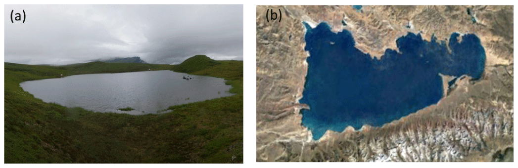
Figure 1(a) Fog3 Lake and (b) Nam Co (b from © Google Earth).
The boundary layer depth depends mainly on the buoyancy and horizontal water flow velocity profiles. In order to compute the boundary layer depth, the bulk Richardson number is first computed as follows:
where Rib is the bulk Richardson number, and B is the buoyancy. When Rib is equal to 0.25 (Kunze et al., 1990; Peters et al., 1995), the shallowest water depth (d) is treated as the depth of the lake boundary layer. The subscript “r” represents the near-surface water layer with a depth of 0.1 m (Br, B(d), ; see the Appendix).
In this study, KPP was implemented into the CLM lake model (CLM-KPP) to improve lake mixing process simulations. In KPP, eddy diffusivity is estimated separately for the lake boundary layer and lake interior. In the lake boundary layer, the eddy diffusivity is determined not by the local gradient of mean variables, but by surface forcing and the boundary layer depth. The non-local effect is taken into account by estimating the boundary layer depth first, and eddy diffusivity is then specified with a prescribed profile in the lake boundary layer. In the lake interior, mixing is associated with internal wave activity and shear instability. However, CLM-ORG does not consider a boundary layer for eddy development, and insufficient water mixing is enhanced through an ad hoc parameter, which is often unable to reflect reality (Zhang et al., 2018). Thus, the coupling of CLM-KPP is essential for better understanding of lake mixing processes.
2.2 Study area
We selected two lakes with available data to evaluate the original lake mixing scheme and KPP. Fog3 Lake is in Arctic Alaska at 68.67∘ N, 149.10∘ W (Fig. 1a). In 2018 it had a surface area of 38 863 m2 and a maximum depth of 21 m. The lake has a long ice duration, and ice-off is usually in late June, while ice-on typically occurs in early October (Arp et al., 2015). Around this lake, the mean annual air temperature is ∘C, and the mean annual precipitation is ∼200 mm (Ping et al., 1998). This kettle lake is surrounded by lower hills covered mainly with shrubs and tundra. Due to the treeless landscape, there are no shielding effects on the wind. In addition, Fog3 Lake is formed by glaciers and has less connection to other surrounding surface waters. The second lake is Nam Co, the highest and largest lake in the central TP (Fig. 1b from © Google Earth). It is situated over 30.5–30.95∘ N, 90.2–91.05∘ E with an altitude of 4730 m and a surface area of about 2021 km2 in 2010 (Lei et al., 2013; Zhu et al., 2010). Its maximum depth reaches more than 95 m, and the mean depth is about 40 m (Wang et al., 2009). The main water supply to Nam Co is precipitation and melting glaciers. Nam Co is a closed lake with no outflow, and water loss occurs mainly through evaporation (Ma et al., 2016).
2.3 Data
Observed hourly meteorological station data for Fog3 Lake were used to drive CLM-ORG and CLM-KPP. Fog3 Lake is about 1.5 km from Toolik Field Station (68∘37.796′ N, 149∘35.834′ W), in the northern foothills of the Brooks Mountain Range, Alaska (https://toolik.alaska.edu/edc/abiotic_monitoring/index.php, last access: 8 October 2019). The forcing variables include downward shortwave and longwave radiation, wind speed, air temperature, air pressure, and specific humidity. Observed lake temperatures from 1 July through 31 August 2018 are for lake depths of 0, 1, 2, 3, 4, 5, 6, 7, 8, 10, 12, 14, and 16 m for model initialization and evaluation.
For Nam Co, the forcing data were from the gridded China meteorological dataset developed by the hydro-meteorological research group at the Institute of Tibetan Plateau Research, Chinese Academy of Sciences (ITPCAS) (Chen et al., 2011; He and Yang, 2011). The forcing variables in this dataset are the same as those for the Alaskan lake. The ITPCAS data cover the period 1979–2015 with a spatial resolution of 0.1∘ and a time step of 3 h. We used the Nam Co meteorological station data for the period of October 2005 through December 2010 to assess the ITPCAS forcing variables. These forcing variables agreed very well with the Nam Co station data, except that the wind speed showed significant biases (Figs. not shown). Linear regression with the station wind speed was applied to correct these biases. Monthly Moderate Resolution Imaging Spectroradiometer (MODIS) surface temperature data at a spatial resolution of 0.05∘ (Savtchenko et al., 2004; Wan et al., 2010) were applied to evaluate the model results for Nam Co. Previous studies have verified MODIS WST data for lakes with in situ observations (Crosman and Horel, 2009; Schneider et al., 2009). Zhang et al. (2014) found that the nighttime WST of MODIS for Nam Co had a 0.89 correlation coefficient and a −1.4 ∘C bias when compared with surface observations. All these studies show that the MODIS WST has acceptable accuracy for studying lake thermal processes.
2.4 Experiment design
Simulations for Fog3 Lake were conducted with both CLM-ORG and CLM-KPP from 1 July through 31 August 2018. The depth for this lake was set at 20 m in both models. Observed lake temperatures for Fog3 Lake are for lake depths of 0, 1, 2, 3, 4, 5, 6, 7, 8, 10, 12, 14, and 16 m. The lake model has 10 lake layers by default, and the center point depths of these layers are 0.05, 0.3, 0.9, 1.9, 3.3, 5.1, 7.5, 10.3, 13.79, and 17.94 m, generated automatically by the layering scheme in the model based on the input lake depth. For this study, we tried to keep each layer thin in the top part of the lake to reflect diurnal cycles (layers 1–5) in both CLM-ORG and CLM-KPP. Below layer 5, we used mostly the observed points to layer the rest of the lake column. Finally, we produced 24 layers for the entire lake column in both models, and the center point depths of these lake layers are 0.05, 0.15, 0.25, 0.35, 0.45, 1, 2, 3, 4, 5, 6, 7, 8, 9, 10, 11, 12, 13, 14, 15, 16, 17, 18, and 19.25 m, respectively. The lake temperatures were initialized with observations for 1 July 2018. The WST and temperature profile simulations with CLM-ORG and CLM-KPP were compared with the observed lake temperatures. For Nam Co, we also used 10 default layers for lake depths in our models without observed vertical temperature profiles, and lake depths were set based on observations (Wang et al., 2009), which ranged from 20 to 95 m. There were 34 model grid cells covering Nam Co with a spatial resolution of 0.1∘. The temperature of each layer was initialized with 277 K. The simulated period for Nam Co was from 2001 through 2012. The simulations for the first two years were discarded as model spin-up, and the remaining simulations were used for analysis. The metrics used for evaluating the performance of the model included the root mean square error (RMSE) and correlation coefficient (R).
3.1 Simulations for Fog3 Lake with CLM-ORG and CLM-KPP
WST simulations with CLM-KPP were more accurate than those with CLM-ORG, especially in August. The RMSE of WST decreased from 0.8 ∘C with CLM-ORG to 0.4 ∘C with CLM-KPP (Fig. 2). CLM-KPP also produced better vertical lake temperature profile simulations than CLM-ORG, particularly in mid-August to late August. The observations showed that the lake mixed on 16 August (Fig. 3a). CLM-KPP accurately captured the mixing event (Fig. 3c), while CLM-ORG produced strong stratification in the upper part of the lake throughout the simulation period (Fig. 3b). Insignificant differences were seen between CLM-ORG and CLM-KPP when compared to observations for the period before 16 August (Table 1), while remarkable improvements were achieved with CLM-KPP during 16–31 August after a strong wind event occurred (Fig. 3d and e). The RMSE of the temperature profile simulations decreased from 1.4 ∘C with CLM-ORG to 0.3 ∘C with CLM-KPP, and R increased from 0.57 to 0.99 for 16–31 August 2018 (Table 1). In general, CLM-KPP had superior performance in simulating well-mixed conditions when compared with CLM-ORG, indicating a successful implementation of KPP into CLM.
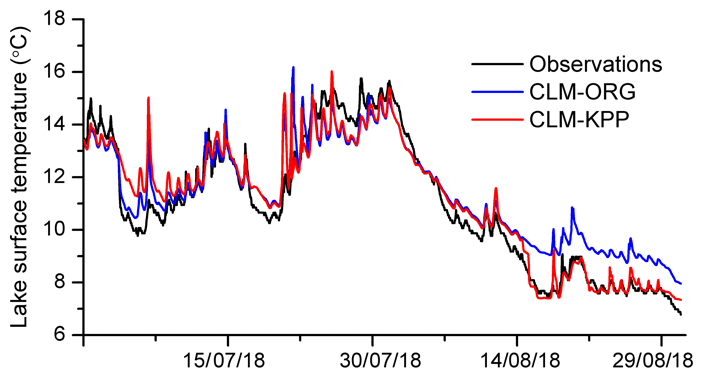
Figure 2WST observations (black line) and simulations with CLM-ORG (blue line) and CLM-KPP (red line) (unit: ∘C).

Figure 3Lake temperature profiles of (a) observations and simulations with (b) CLM-ORG and (c) CLM-KPP. Lake temperature profile differences between simulations and observations: (d) CLM-ORG minus observations and (e) CLM-KPP minus observations (unit: ∘C).
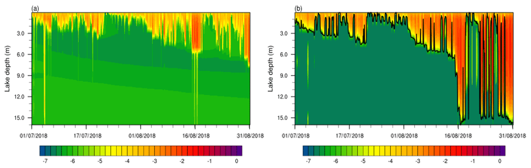
Figure 4Simulated (a) with CLM-ORG, and (b) with CLM-KPP (unit: m2 s−1). The black line in (b) shows the lake boundary layer depth (unit: m).
Table 1RMSE (∘C) and R of temperature profile simulations with CLM-ORG and CLM-KPP for Fog3 Lake for the periods of 1 July–15 August, and 16–31 August 2018.
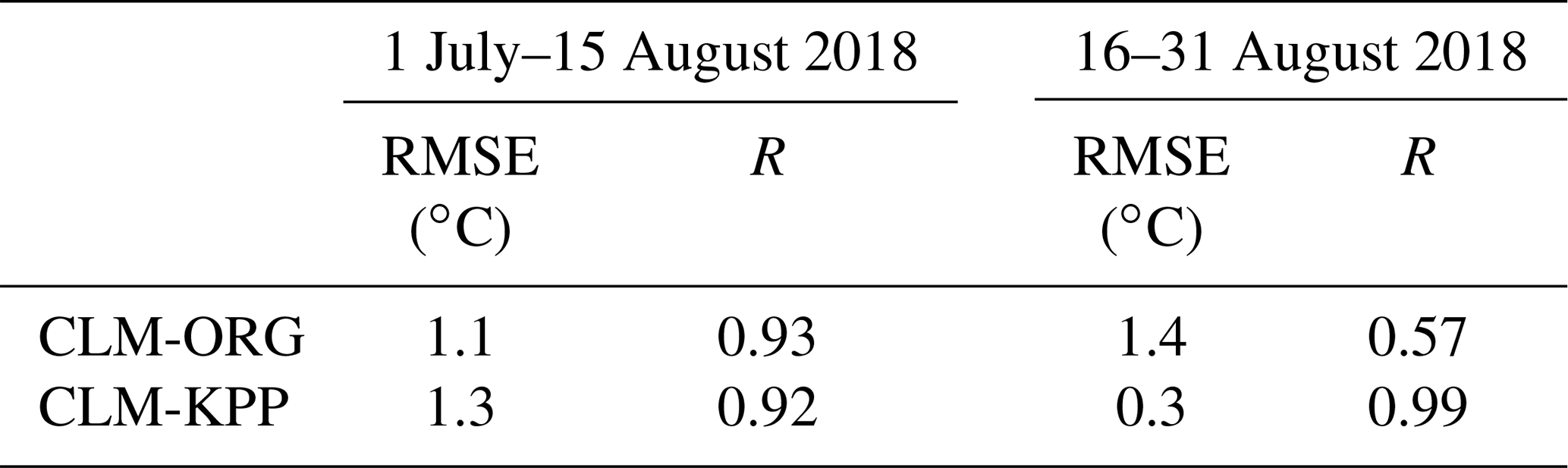
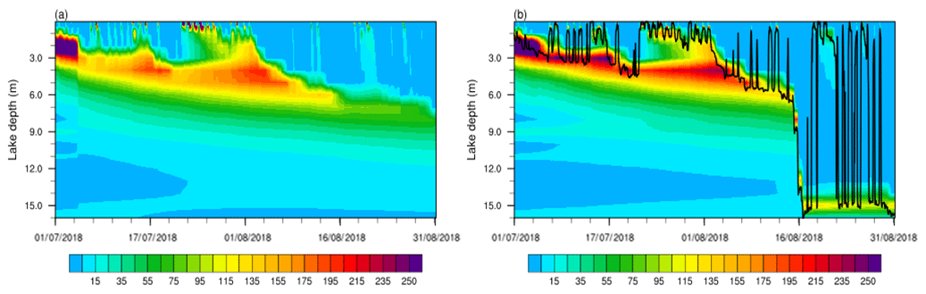
Figure 5Simulated N2 with (a) CLM-ORG and (b) CLM-KPP (unit: 10−5 s−2). The black line in (b) shows the lake boundary layer depth (unit: m).
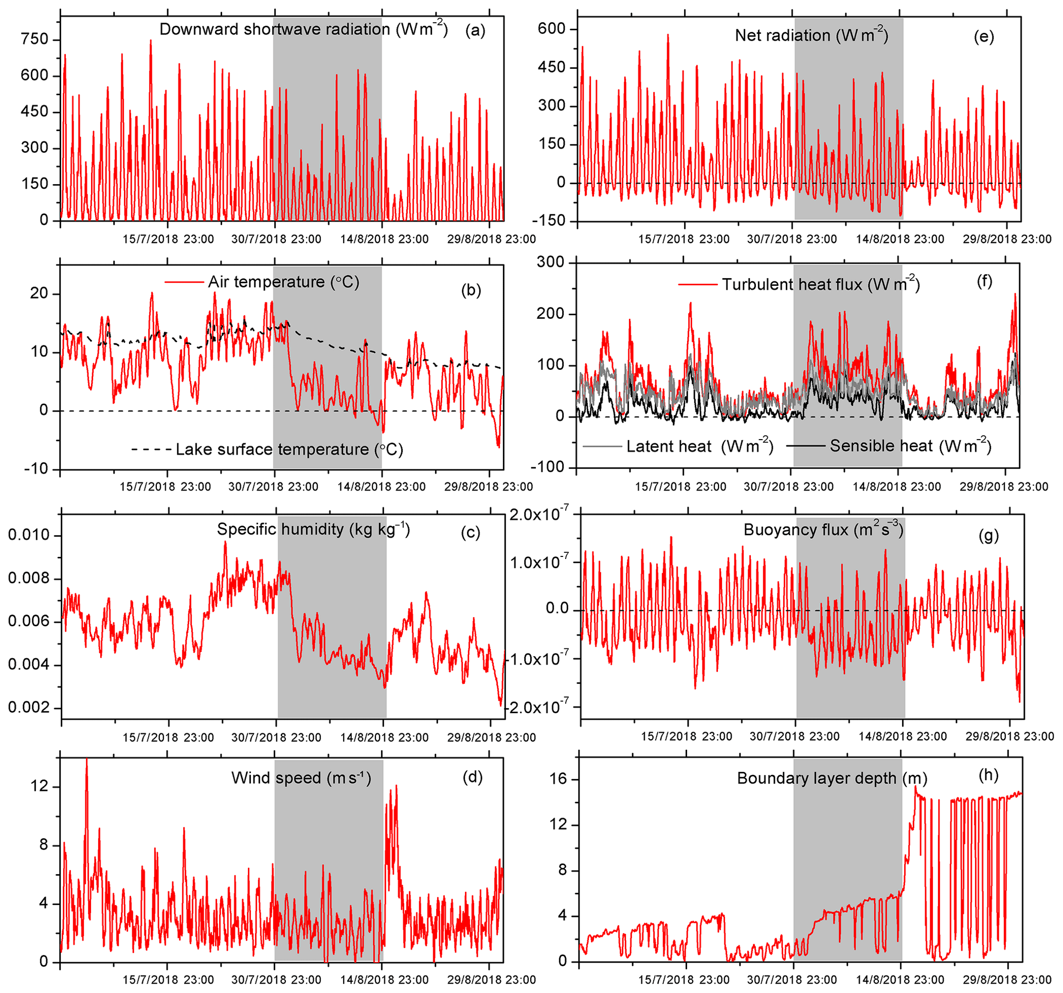
Figure 6Time series of (a) observed downward shortwave radiation (W m−2), (b) observed air temperature and WST (∘C), (c) observed specific humidity (kg kg−1), (d) observed wind speed (m s−1), (e) simulated net radiation (W m−2), (f) simulated turbulent heat flux (W m−2) (red line) with latent heat flux (gray line) and sensible heat flux (black line), (g) simulated buoyancy flux (m2 s−3), and (h) simulated boundary layer depth (m). The gray shading covers 1 through 15 August. The simulations were from CLM-KPP.
Simulations of total diffusivity (m2 s−1) with CLM-KPP were compared with those of with CLM-ORG. within the boundary layer was generally larger than , especially in August (Fig. 4). However, the total diffusivity with CLM-ORG was higher than that with CLM-KPP below the boundary layer (Fig. 4). The pattern of the diffusivity with CLM-ORG was consistent with that of the squared buoyancy frequency N2 (Fig. 5), implying that the enhanced diffusivity (Ked) was weighted very highly in in this model. In the meantime, was mostly on the order of 10−7 m2 s−1 and was the sum of internal-wave diffusivity, molecular diffusivity, and diffusivity due to shear instability (Eq. 14). The first two terms were also on the order of 10−7 m2 s−1, indicating that the total diffusivity with CLM-KPP was controlled mostly by these two terms. In early July, sometimes appeared to be on the order of 10−5 m2 s−1, which was consistent with that of the last term, shear instability diffusivity, implying that this term dominated . The diffusivity increase was closely related to the strong winds occurring at the same time (Fig. 4b).
The squared buoyancy frequency N2 of simulations with both CLM-KPP and CLM-ORG were also compared for our study period. N2 was related to the water density gradient (Eq. 6) determined by the temperature gradient in both models. A greater N2 produced more stable water and stronger water stratification. From 1 July through 15 August, the simulated N2 with CLM-KPP near the bottom of the boundary layer was slightly larger than that with CLM-ORG (Fig. 5). Thus, the simulated water stratification with CLM-KPP at the bottom of the boundary layer was stronger than that in CLM-ORG before 16 August. However, after 16 August, the maximum N2 with CLM-ORG occurred in the middle layer of the lake, maintaining stratification there. Conversely, the maximum N2 with CLM-KPP moved down to near the bottom of the lake during the same 16 d period (Fig. 5).
3.2 Analysis of CLM-KPP simulations for Fog3 Lake
We examined our simulations and meteorological forcing data in detail to physically understand water mixing conditions simulated by CLM-KPP, especially over the period of 16–31 August 2018. Figure 6a shows that downward shortwave radiation was 45 W m−2 lower during 1–15 August (shaded area) than in July. Meanwhile, over the same period, air temperature and specific humidity decreased dramatically, while wind speed showed almost no trend (Fig. 6b–d). In this period, the simulated net radiation with CLM-KPP was 54 W m−2 lower than that for July (Fig. 6e). The turbulent heat flux, the sum of sensible and latent heat fluxes, increased over this 15 d period due mainly to the decreased air temperature and humidity (Fig. 6f). Figure 6g shows that buoyancy flux, defined as net radiation minus turbulent heat flux in the boundary layer with a different unit (m2 s−3), was mostly negative during 1–15 August, showing that the lake was losing heat. Due to this heat loss, the temperature in the upper lake decreased, reducing the temperature difference between the upper and lower parts of the lake and thus weakening the stratification. Therefore, we can see that the boundary layer depth increased over the period of 1–15 August (Fig. 6h) when the wind had no systematic changes, but the buoyancy flux played a significant role in this increase.

Figure 7Time series over the period of 2003 through 2012 of monthly WST observations from MODIS (black starred line) and simulations with CLM-ORG (blue line) and CLM-KPP (red line) (unit: ∘C).
During 15–16 August, a wind event (12 m s−1) mixed the lake, dramatically increasing the boundary layer depth in addition to the negative buoyancy flux. The deep boundary layer was maintained through the end of August, even though the winds returned to normal conditions. Such strong mixing was not seen in CLM-ORG, where the water stratification could not be broken up by the high wind event without help from the negative buoyancy flux. Hence, without an ad hoc parameter to enhance the water diffusivity as in CLM-ORG, CLM-KPP still reproduced the observed water mixing processes.
3.3 Model validation with Nam Co data
We validated both CLM-ORG and CLM-KPP with MODIS data for Nam Co by conducting 10 km spatial resolution simulations for this lake over the period of 2003 through 2012. We can see that CLM-KPP improved WST simulations averaged over the entire lake (34 model grid cells) when compared with the MODIS data and CLM-ORG simulations (Fig. 7). The RMSE of WST decreased from 4.58 ∘C with CLM-ORG to 2.23 ∘C with CLM-KPP, and R increased from 0.90 to 0.96 at the same time.
The improved WST simulations with CLM-KPP were closely related to the water diffusivity simulations with KPP as discussed above. We averaged the and simulations over water columns with depth greater than 25 m for Nam Co, as shown in Fig. 8, and the total of such columns was 28 out of 34 for this lake. Figure 8 indicates that was slightly smaller than , mostly in the mixing layer of the lake, over the summer. The difference likely resulted from the enlarged in CLM where this parameter was increased by a factor of 10 when the lake depth was greater than 25 m. In the deeper part of the lake, was much smaller than over the summer due much to the contribution of Ked to . In the spring and fall, was significantly larger than . During the winter when the lake froze, both CLM-KPP and CLM-ORG were set to use . We can see that the most significant improvements in WST for Nam Co occurred during the ice-free seasons when KPP was activated. Overall, CLM-KPP can enhance the water diffusivity during spring and fall and maintain weak water diffusivity in the lake interior during summer when stratification is strong.
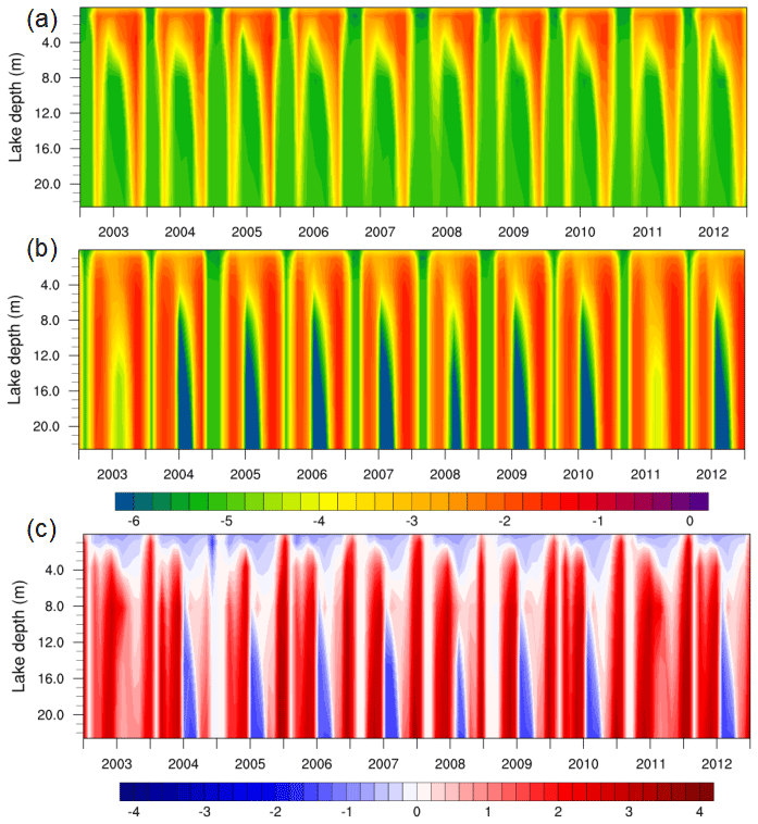
Figure 8Simulated (a) with CLM-ORG, (b) with CLM-KPP (unit: m2 s−1) averaged over water columns with depth greater than 25 m (28 of 34 grid cells), and (c) differences between and ().
We improved lake mixing process simulations by applying the vertical mixing scheme KPP in CLM. The improved lake model was applied to an Arctic Alaskan lake and to Nam Co lake in the TP for model evaluation. Results for the Alaskan lake indicate that the WST and lake temperature profile simulations using KPP are greatly improved when compared to the original vertical mixing scheme in CLM. During the transition season in August, the improvement is most obvious. This improvement is associated with negative heat flux and high wind, which can cause deepening of the boundary layer and strong mixing. However, the original vertical mixing scheme of CLM cannot capture these strong mixing events and causes a positive lake temperature bias in its simulation. CLM-KPP was further validated with the observed data from Nam Co, and results showed that WST simulations were significantly improved when compared with the MODIS data and CLM-ORG simulations.
More data are needed to further verify CLM-KPP, including atmospheric forcing data over lakes and observed lake temperature profiles. It should also be noted that although CLM-KPP has improved thermal process simulations, large WST biases still existed during the ice freezing period for Nam Co. Such biases most likely resulted from the oversimplified lake ice scheme in the CLM lake model. Therefore, a more realistic ice scheme in lake models is needed for better understanding of the effects of water mixing on ice formation. In general, this coupled model provides an important tool for lake hydrology and ecosystem studies.
The model configuration and input data used in this study are available upon request.
Lake temperature is calculated as follows:
where T is lake temperature (K) at depth z (m) and time t (s), ϕ is the absorbed solar radiation flux as a heat source term (W m−2), Cw is the volumetric heat capacity of lake water (J m−3 K−1), and Kw is the total diffusivity (m2 s−1).
The non-dimensional flux profiles are calculated as follows:
The non-dimensional shape function G(σ) is a third-order polynomial:
a0, a1, a2, and a3 are given as follows:
where υ(h) is the total diffusivity as a function of lake depth (h), w(1) is the velocity scale at the bottom of the lake boundary layer, ∂υ(h) is the lake depth derivative of υ, and ∂w(1) is the lake depth derivative of w at the bottom of the lake boundary layer.
B(d) is the buoyancy calculated with a depth of d as follows:
is calculated as follows:
where Ric=0.25, Cv=1.6, βT=0.2, and .
QZ conducted the modeling, performed the analysis, and drafted the paper. JJ designed the study, interpreted the results, and supervised the research. XW contributed the original ideas of the research. PB and NB provided observational data and helped with the study design and data analysis. SEN gave constructive comments on the results. All authors edited the paper.
The authors declare that they have no conflict of interest.
This article is part of the special issue “Modelling lakes in the climate system (GMD/HESS inter-journal SI)”. It is a result of the 5th workshop on “Parameterization of Lakes in Numerical Weather Prediction and Climate Modelling”, Berlin, Germany, 16–19 October 2017.
This work was supported by the National Natural Science Foundation of China (grant numbers 91637209, 41571030, and 91737306) and a grant from the US National Science Foundation (grant number 1603088). Qunhui Zhang was also supported by the National Key R & D Program of China on monitoring, early warning, and prevention of major natural disasters (no. 2018YFC150703). Jiming Jin was also supported by Utah Agricultural Experiment Station. The gridded meteorological dataset for China used in this study as forcing data was accessible from the Third Pole Environment Database (http://en.tpedatabase.cn/portal/MetaDataInfo.jsp?MetaDataId=202, last access: 29 November 2017). The MODIS lake temperature data products (MOD11 and MYD11) were from https://modis.gsfc.nasa.gov/data/dataprod (last access: 20 September 2018). The Nam Co station data were from http://www.tpedatabase.cn) (last access: 17 January 2019).
This research has been supported by the National Natural Science Foundation of China (grant nos. 91637209, 41571030, and 91737306) and the US National Science Foundation (grant no. 1603088). Qunhui Zhang was also supported by the National Key R & D Program of China on monitoring, early warning, and prevention of major natural disasters (grant no. 2018YFC150703). Jiming Jin was also supported by Utah Agricultural Experiment Station.
This paper was edited by Miguel Potes and reviewed by two anonymous referees.
Arp, C. D., Jones, B. M., Liljedahl, A. K., Hinkel, K. M., and Welker, J. A.: Depth, ice thickness, and ice-out timing cause divergent hydrologic responses among Arctic lakes, Water Resour. Res., 51, 9379–9401, https://doi.org/10.1002/2015WR017362, 2015.
Banks, R. B.: Some features of wind action in shallow lakes, Proc. Am. Soc. Civ. Eng., 101, 813–827, 1975.
Berger, S. A., Diehl, S., Kunz, T. J., Albrecht, D., Oucible, A. M., and Ritzer, S.: Light supply, plankton biomass, and seston stoichiometry in a gradient of lake mixing depths, Limnol. Oceanogr., 51, 1898–1905, https://doi.org/10.4319/lo.2006.51.4.1898, 2006.
Bonan, G. B.: Sensitivity of a GCM simulation to inclusion of inland water surface, J. Climate, 8, 2691–2704, https://doi.org/10.1175/1520-0442(1995)008<2691:SOAGST>2.0.CO;2, 1995.
Bryson, R. A. and Ragotzkie, R. A.: On internal waves in lakes, Limnol. Oceanogr., 5, 397–408, https://doi.org/10.4319/lo.1960.5.4.0397, 1960.
Budy, P. and Luecke, C.: Understanding how lake populations of arctic char are structured and function with special consideration of the potential effects of climate change: A multi-faceted approach, Oecologia, 176, 81–94, https://doi.org/10.1007/s00442-014-2993-8, 2014.
Chen, Y., Yang, K., He, J., Qin, J., Shi, J., Du, J., and He, Q.: Improving land surface temperature modeling for dry land of China, J. Geophys. Res.-Atmos., 116, D20104, https://doi.org/10.1029/2011JD015921, 2011.
Chiswell, S. M.: Annual cycles and spring blooms in phytolankton: Don't abandon Sverdrup completely, Mar. Ecol.-Prog. Ser., 443, 39–50, 2011.
Crosman, E. T. and Horel, J. D.: MODIS-derived surface temperature of the Great Salt Lake, Remote Sens. Environ., 113, 73–81, https://doi.org/10.1016/j.rse.2008.08.013, 2009.
Dai, Y., Yao, T., Li, X., and Ping, F.: The impact of lake effects on the temporal and spatial distribution of precipitation in the Nam Co basin, Tibetan Plateau, Quatern. Int., 475, 63–69, https://doi.org/10.1016/j.quaint.2016.01.075, 2018.
Diallo, I., Giorgi, F., and Stordal, F.: Influence of Lake Malawi on regional climate from a double-nested regional climate model experiment, Clim. Dynam., 50, 3397–3411, https://doi.org/10.1007/s00382-017-3811-x, 2018.
Dodson, S. I.: Introduction to limnology, J. N. Am. Benthol. Soc., 23, 661–662, https://doi.org/10.1899/0887-3593(2004)023<0661:ITL>2.0.CO;2, 2004.
Etemad-Shahidi, A. and Imberger, J.: Diapycnal mixing in the thermocline of lakes: Estimation by different methods, Environ. Fluid Mech., 6, 227–240, https://doi.org/10.1007/s10652-005-4480-6, 2006.
Fang, X. and Stefan, H. G.: Long-term lake water temperature and ice cover simulations/measurements, Cold Reg. Sci. Technol., 24, 289–304, https://doi.org/10.1016/0165-232X(95)00019-8, 1996.
Foley, B., Jones, I. D., Maberly, S. C., and Rippey, B., Long-term changes in oxygen depletion in a small temperate lake: Effects of climate change and eutrophication, Freshwater Biol., 57, 278–289, https://doi.org/10.1111/j.1365-2427.2011.02662.x, 2012.
Goudsmit, G. H., Burchard, H., Peeters, F., and Wüest, A.: Application of k−ε turbulence models to enclosed basins: The role of internal seiches, J. Geophys. Res.-Oceans, 107, 3230, https://doi.org/10.1029/2001JC000954, 2002.
Gu, H., Jin, J., Wu, Y., Ek, M. B., and Subin, Z. M.: Calibration and validation of lake surface temperature simulations with the coupled WRF-lake model, Climatic Change, 129, 471–483, https://doi.org/10.1007/s10584-013-0978-y, 2013.
Gu, H., Ma, Z., and Li, M.: Effect of a large and very shallow lake on local summer precipitation over the Lake Taihu basin in China, J. Geophys. Res.-Atmos., 121, 8832–8848, https://doi.org/10.1002/2015JD024098, 2016.
He, J. and Yang, K.: China Meteorological Forcing Dataset, Cold and Arid Regions Science Data Center, Lanzhou, https://doi.org/10.3972/westdc.002.2014.db, 2011.
Henderson-Sellers, B.: New formulation of eddy diffusion thermocline models, Appl. Math. Model., 9, 441–446, https://doi.org/10.1016/0307-904X(85)90110-6, 1985.
Hostetler, S. W. and Bartlein, P. J.: Simulation of lake evaporation with application to modeling lake level variations of Harney-Malheur Lake, Oregon, Water Resour. Res., 26, 2603–2612, https://doi.org/10.1029/WR026i010p02603, 1990.
Jeffries, M. O., Zhang, T., Frey, K., and Kozlenko, N.: Estimating late-winter heat flow to the atmoshere from the lake-dominated Alaskan north slope, J. Glaciol., 45, 315–324, https://doi.org/10.3189/S0022143000001817, 1999.
Kheyrollah Pour, H., Duguay, C. R., Martynov, A., and Brown, L. C.: Simulation of surface temperature and ice cover of large northern lakes with 1-D models: A comparison with MODIS satellite data and in situ measurements, Tellus A, 64, 17614, https://doi.org/10.3402/tellusa.v64i0.17614, 2012.
Krinner, G.: Impact of lakes and wetlands on boreal climate, J. Geophys. Res., 108, 4520, https://doi.org/10.1029/2002JD002597, 2003.
Kunze, E., Williams, A. J., and Briscoe, M. G.: Observations of shear and stability from a neutrally buoyant float, J. Geophys. Res., 95, 18127–18142, https://doi.org/10.1029/JC095iC10p18127, 1990.
Laird, N. F., Desrochers, J., and Payer, M.: Climatology of lake-effect precipitation events over Lake Champlain, J. Appl. Meteorol. Clim., 48, 232–250, https://doi.org/10.1175/2008JAMC1923.1, 2009.
Large, W. G. and Pond, S.: Sensible and latent heat flux measurements over the ocean, J. Phys. Oceanogr., 12, 464–482, https://doi.org/10.1175/1520-0485(1982)012<0464:SALHFM>2.0.CO;2, 1982.
Large, W. G., McWilliams, J. C., and Doney, S. C.: Oceanic vertical mixing: A review and a model with a nonlocal boundary layer parameterization, Rev. Geophys., 32, 363–403, https://doi.org/10.1029/94RG01872, 1994.
Lei, Y., Yao, T., Bird, B. W., Yang, K., Zhai, J., and Sheng, Y.: Coherent lake growth on the central Tibetan Plateau since the 1970s: Characterization and attribution, J. Hydrol., 483, 61–67, https://doi.org/10.1016/j.jhydrol.2013.01.003, 2013.
Li, X., Chao, Y., McWilliams, J. C., and Fu, L. L.: A comparison of two vertical-mixing schemes in a Pacific Ocean General Circulation Model, J. Climate, 14, 1377–1398, https://doi.org/10.1175/1520-0442(2001)014<1377:ACOTVM>2.0.CO;2, 2001.
Lofgren, B. M.: A model for simulation of the climate and hydrology of the Great Lake basin, J. Geophys. Res., 109, D18108, https://doi.org/10.1029/2004JD004602, 2004.
Long, Z., Perrie, W., Gyakum, J., Caya, D., and Laprise, R.: Northern lake impacts on local seasonal climate, J. Hydrometeorol., 8, 881–896, https://doi.org/10.1175/JHM591.1, 2007.
Ma, N., Szilagyi, J., Niu, G.-Y., Zhang, Y., Zhang, T., Wang, B., and Wu, Y.: Evaporation variability of Nam Co Lake in the Tibetan Plateau and its role in recent rapid lake expansion, J. Hydrol., 537, 27–35, https://doi.org/10.1016/j.jhydrol.2016.03.030, 2016.
Mahadevan, A., D'Asaro, E., Lee, C., and Perry, M. J.: Eddy-driven stratification initiates North Atlantic spring phytoplankton blooms, Science, 337, 54–58, https://doi.org/10.1126/science.1218740, 2012.
Marshall, B. E., Ezekiel, C. N., Gichuki, J., Mkumbo, O. C., Sitoki, L., and Wanda, F.: Has climate change disrupted stratification patterns in Lake Victoria, East Africa?, Afr. J. Aquat. Sci., 38, 249–253, https://doi.org/10.2989/16085914.2013.810140, 2013.
Martynov, A., Sushame, L., and Laprise, R.: Simulations of temperate freezing lakes by one-dimensional lake models: Performance assessment for interactive coupling with regional cliamte models, Boreal Environ. Res., 15, 143–164, 2010.
Michalski, J. and Lemmin, U.: Dynamics of vertical mixing in the hypolimnion of a deep lake: Lake Geneva, Limnol. Oceanogr., 40, 809–816, https://doi.org/10.4319/lo.1995.40.4.0809, 1995.
Mironov, D. V.: Parameterization of lakes in numerical weather prediction. Description of a lake model, COSMO Technology Report 11[R], Deutscher Wetterdienst, Offenbach am Main, Germany, 2008.
Monin, A. S. and Obukhov, A. M.: Basic laws of turbulent mixing in the atmospheric near the ground, Akad. Naud. SSSR Geofiz. Inst., 24, 163–187, 1954.
O'Brien, W. J., Barfield, M., Bettez, N., Hershey, A. E., Hobbie, J. E., Kipphut, G., Kling, G., and Miller, M. C.: Long-term response and recovery to nutrient addition of a partitioned arctic lake, Freshwater Biol., 50, 731–741, https://doi.org/10.1111/j.1365-2427.2005.01354.x, 2005.
Oleson, K., Lawrence, D. M., Bonan, G. B., Drewniak, B., Huang, M., Koven, C. D., Levis, S., Li, F., Riley, W. J., Subin, Z. M., Swenson, S., Thornton, P. E., Bozbiyik, A., Fisher, R., Heald, C. L., Kluzek, E., Lamarque, J. F., Lawrence, P. J., Leung, L. R., Lipscomb, W., Muszala, S. P., Ricciuto, D. M., Sacks, W. J., Sun, Y., Tang, J., and Yang, Z.: Technical description of version 4.5 of the Community Land Model (CLM), NCAR Technical Note NCAR/TN-503+STR, NCAR, Boulder, Colorado, 420 pp., https://doi.org/10.5065/D6RR1W7M, 2013.
Perroud, M., Goyette, S., Martynov, A., Beniston, M., and Anneville, O.: Simulation of multiannual thermal profiles in deep Lake Geneva: A comparison of one-dimensional lake models, Limnol. Oceanogr., 54, 1574–1594, https://doi.org/10.4319/lo.2009.54.5.1574, 2009.
Peters, H., Gregg, M. C., and Sanford, T. B.: On the parameterization of equatorial turbulence: Effect of fine-scale variations below the range of the diurnal cycle, J. Geophys. Res., 100, 18333–18348, https://doi.org/10.1029/95JC01513, 1995.
Ping, C. L., Bockheim, J. G., Kimble, J. M., Michaelson, G. J., and Walker, D. A.: Characteristics of cryogenic soils along a latitudinal transect in arctic Alaska, J. Geophys. Res., 103, 28917–28928, https://doi.org/10.1029/98JD02024, 1998.
Powell, T. and Jassby, A.: The estimation of vertical eddy diffusivities below the thermocline in lakes, Water Resour. Res., 10, 191–198, https://doi.org/10.1029/WR010i002p00191, 1974.
Roekel, L. P. V., Adcroft, A. J., Danabasoglu, G., Griffies, S. M., Kauffman, B., Large, W., Levy, M., Reichl, B., Ringler, T., and Schmidt, M.: The KPP boundary layer scheme: Revisiting its formulation and benchmarking one-dimensional ocean simulations relative to LES, J. Adv. Model. Earth Syst., 10, 2647–2685, https://doi.org/10.1029/2018MS001336, 2018.
Rouse, W. R., Oswald, C. J., Binyamin, J., Spence, C., Schertzer, W. M., Blanken, P. D., Bussieres, N., and Duguay, C. R.: The role of northern lakes in a regional energy balance, J. Hydrometeorol., 6, 291–305, https://doi.org/10.1175/JHM421.1, 2005.
Rouse, W. R., Blanken, P. D., Bussières, N., Walker, A. E., Oswald, C. J., Schertzer, W. M., and Spence, C.: An investigation of the thermal and energy balance regimes of Great Slave and Great Bear Lakes, J. Hydrometeorol., 9, 1318–1333, https://doi.org/10.1175/2008JHM977.1, 2008.
Samuelsson, P., Kourzeneve, E., and Mironov, D.: The impact of lakes on the European climate as simulated by a regional climate model, Boreal Environ. Res., 15, 113–129, 2010.
Savtchenko, A., Ouzounov, D., Ahmad, S., Acker, J., Leptoukh, G., Koziana, J., and Nickless, D.: Terra and Aqua MODIS products available from NASA GES DAAC, Adv. Space Res., 34, 710–714, https://doi.org/10.1016/j.asr.2004.03.012, 2004.
Schneider, P., Hook, S. J., Radocinski, R. G., Corlett, G. K., Hulley, G. C., Schladow, S. G., and Steissberg, T. E.: Satellite observations indicate rapid warming trend for lakes in California and Nevada, Geophys. Res. Lett., 36, L22402, https://doi.org/10.1029/2009GL040846, 2009.
Shchepetkin, A. F. and McWilliams, J. C.: The regional oceanic modeling system (ROMS): A split-explicit, free-surface, topography-following-coordinate oceanic model, Ocean Model., 9, 347–404, https://doi.org/10.1016/j.ocemod.2004.08.002, 2005.
Shimoda, Y., Azim, M. E., Perhar, G., Ramin, M., Kenney, M. A., Sadraddini, S., Gudimov, A., and Arhonditsis, G. B.: Our current understanding of lake ecosytem response to climate change: What have we really learned from the north temperate deep lakes?, J. Great Lakes Res., 37, 173–193, https://doi.org/10.1016/j.jglr.2010.10.004, 2011.
Stanichny, S. V., Kubryakov, A. A., and Soloviev, D. M.: Parameterization of surface wind-driven currents in the Black Sea using drifters, wind, and altimetry data, Ocean Dynam., 66, 1–10, https://doi.org/10.1007/s10236-015-0901-3, 2016.
Stepanenko, V. M., Goyetter, S., Martynov, A., Perroud, M., Fang, X., and Mironov, D.: First steps of a Lake Model Intercomparison Project LakeMIP, Boreal Environ. Res., 15, 191–202, 2010.
Stepanenko, V. M., Martynov, A., Jöhnk, K. D., Subin, Z. M., Perroud, M., Fang, X., Beyrich, F., Mironov, D., and Goyette, S.: A one-dimensional model intercomparison study of thermal regime of a shallow, turbid midlatitude lake, Geosci. Model Dev., 6, 1337–1352, https://doi.org/10.5194/gmd-6-1337-2013, 2013.
Stepanenko, V. M., Jöhnk, K. D., Machulskaya, E., Perroud, M., Subin, Z., Nordbo, A., Mammarella, I., and Mironov, D.: Simulation of surface energy fluxes and stratification of a small boreal lake by a set of one-dimensional models, Tellus A, 66, 21389, https://doi.org/10.3402/tellusa.v66.21389, 2014.
Stepanenko, V. M., Mammarella, I., Ojala, A., Miettinen, H., Lykosov, V., and Vesala, T.: LAKE 2.0: A model for temperature, methane, carbon dioxide and oxygen dynamics in lakes, Geosci. Model Dev., 9, 1977–2006, https://doi.org/10.5194/gmd-9-1977-2016, 2016.
Subin, Z. M., Riley, W. J., and Mironov, D.: An improved lake model for climate simulations: Model structure, evaluation, and sensitivity analyses in CESM1, J. Adv. Model. Earth Syst., 4, M02001, https://doi.org/10.1029/2011MS000072, 2012.
Sun, X., Xie, L., Semazzi, F., and Liu, B.: Effect of lake surface temperature on the spatial distribution and intensity of the precipitation over the Lake Victoria basin, Mon. Weather Rev., 143, 1179–1192, https://doi.org/10.1175/MWR-D-14-00049.1, 2015.
Sweers, H. E.: Vertical diffusivity coefficient in a thermocline, Limnol. Oceanogr., 15, 273–280, https://doi.org/10.4319/lo.1970.15.2.0273, 1970.
Thiery, W., Davin, E. L., Panitz, H.-J., Demuzere, M., Lhermitte, S., and van Lipzig, N.: The impact of the African Great Lakes on the regional climate, J. Climate, 28, 4061–4085, https://doi.org/10.1175/JCLI-D-14-00565.1, 2015.
Thorpe, S. A. and Jiang, R.: Estimating internal waves and diapycnal mixing from conventional mooring data in a lake, Limnol. Oceanogr., 43, 936–945, https://doi.org/10.4319/lo.1998.43.5.0936, 1998.
Verhagen, J. H. G.: Modeling phytoplankton patchiness under the influence of wind-driven currents in lakes, Limnol. Oceanogr., 39, 1551–1565, https://doi.org/10.4319/lo.1994.39.7.1551, 1994.
Wan, Z., Zhang, Y., Zhang, Q., and Li, Z. L.: Quality assessment and validation of the MODIS global land surface temperature, Int. J. Remote Sens., 25, 261–274, https://doi.org/10.1080/0143116031000116417, 2010.
Wang, J., Zhu, L., Daut, G., Ju, J., Lin, X., Wang, Y., and Zhen, X.: Investigation of bathymetry and water quality of Lake Nam Co, the largest lake on the central Tibetan Plateau, China, Limnology, 10, 149–158, https://doi.org/10.1007/s10201-009-0266-8, 2009.
Wang, X., Yi, C., Zhang, H., Farrara, J., Li, Z., Xin, J., Park, K., Colas, F., McWilliams, J. C., and Paternostro, C.: Modeling tides and their influence on the circulation in Prince William Sound, Alaska, Cont. Shelf Res., 63, S126–S137, https://doi.org/10.1016/j.csr.2012.08.016, 2013.
Wu, J.: Wind-induced drift currents, J. Fluid Mech., 68, 49–70, https://doi.org/10.1017/S0022112075000687, 1975.
Yao, H., Samal, N. R., Joehnk, K. D., Fang, X., Bruce, L. C., Pierson, D. C., Rusak, J. A., and James, A.: Comparing ice and temperature simulations by four dynamic lake models in Harp Lake: Past performance and future predictions, Hydrol. Process., 28, 4587–4601, https://doi.org/10.1002/hyp.10180, 2014.
Zhang, G., Yao, T., Xie, H., Qin, J., Ye, Q., Dai, Y., and Guo, R.: Estimating surface temperature changes of lakes in the Tibetan Plateau using MODIS LST data, J. Geophys. Res.-Atmos., 119, 8552–8567, https://doi.org/10.1002/2014JD021615, 2014.
Zhang, Q., Jin, J., Zhu, L., and Lu, S.: Modelling of water surface temperature of three lakes on the Tibetan Plateau using a physically based lake model, Atmos.-Ocean, 56, 289–295, https://doi.org/10.1080/07055900.2018.1474085, 2018.
Zhu, L., Xie, M., and Wu, Y.: Quantitative analysis of lake area variations and the influence factors from 1971 to 2004 in the Nam Co basin of the Tibetan Plateau, Chin. Sci. Bull., 55, 1294–1303, https://doi.org/10.1007/s11434-010-0015-8, 2010.
Zhu, L., Jin, J., Liu, X., Tian, L., and Zhang, Q.: Simulations of the impact of lakes on local and regional climate over the Tibetan Plateau, Atmos.-Ocean, 56, 230–239, https://doi.org/10.1080/07055900.2017.1401524, 2017.