2.1 From quantile mapping to optimal transport

We start with the construction of a quantile mapping method in the univariate case, i.e., with d=1. In this context, the biased and reference random variables are denoted X and Y, respectively. A transfer function 𝒯 between X and Y is constructed on the cumulative distribution functions (CDFs) of X and Y, defined by

A realization y of Y is the correction of a realization x of X if and only if F_X(x)=F_Y(y). Under the assumption that F_Y is invertible, the correction y of x is given by

Thus the transfer function is written $\mathcal{T}=F_Y^{-\mathrm{1}}\circ F_X$. This method is called quantile mapping. Indeed, the quantiles of X and Y are matched through the relation F_X(x)=F_Y(y).

Figure 1Histogram of two Gaussian laws X and Y in blue and red. (a) The x axis indicates the edges of each bar. The black arrows indicate how the quantile mapping matches an element of X with its correction. (b) The x axis gives the center of each bar. The black arrows indicate the possibilities for how the probability of obtaining the value x₁ for X can be distributed among the possible values y_j of Y. The γ_1j correspond to the number of realizations moved. These arrows can be generalized to each x_i. (c) The x axis gives the center of each bar. The black arrows indicate the non-zero γ_ij estimated by the OTC method. (d) Bivariate histogram of two Gaussian laws. The black arrows represent how the OTC method fits each x_i with its correction. To facilitate readability, only 30 arrows are represented.

Download

We illustrate the quantile mapping method with an example in Fig. 1a. In this example, the random variables X and Y are two Gaussian laws centered, respectively, on 0 and 10, with a standard deviation of 1. We cut ℝ into cells of length 1 and estimate the histograms. Fig. 1a shows the two histograms of X and Y in red and blue, respectively. The x axis gives the empirical quantiles of the edges of each cell. The black arrows indicate how the quantile mapping connects a cell of X to a cell of Y. For example, the realizations of X in the first blue cell are corrected and transferred to realizations in the first three red cells of Y.

The main point here is the following: in the univariate context, we can perform a bias correction with only the black arrows. A realization in a cell of X is corrected to a realization into a cell of Y connected by a black arrow. Because in a multivariate context the quantile mapping can not be used to estimate these arrows (CDFs are not invertible), our problem is the following: how to construct these black arrows in a multivariate context.

For this, let x_i (y_j) be the centers of each cell of the histogram of X (Y). Let p_xi be the number of realizations of X in the interval x_i, and let p_yj be the number of realizations of Y in the interval y_j. We represent all possible black arrows by a collection of coefficients γ_ij. A γ_ij value corresponds to the number of realizations in the cell x_i that are transferred to realizations in the cell y_j. We obtain the following two equalities:

representing how the cell x_j is split into each cell y_j; and

representing how cell y_j received the realizations from each cell x_i. We depict the γ_1j coefficients in Fig. 1b. The black arrows represent the number of realizations γ_1j that are transferred to each y_j.

The problem is to calculate the coefficients γ_ij. For each displacement γ_ij, we can associate a cost, which is the square of the length of the displacement, $|x_i-y_j{|}^{\mathrm{2}}$. This choice comes from the optimal transport theory, and will be highlighted in the next section. To correct γ_ij realizations, we have a cost of ${\mathit{\gamma }}_{ij}|x_i-y_j{|}^{\mathrm{2}}$. We thus obtain a global cost associated with the γ_ij coefficients:

Our bias correction method is defined by the γ_ij coefficients minimizing the functional C. The γ_ij obtained by minimizing C for our example are shown in Fig. 1c. Comparing with the quantile mapping in Fig. 1a, we can see that the obtained coefficients (the black arrows) are similar. Indeed, the coefficients induced by the quantile mapping are precisely those minimizing the functional C. Proofs of this statement can be found in Farchi et al. (2016, Appendix A) and Santambrogio (2015, chap. 2). In other words, even in the absence of CDF, a bias correction can be carried out by calculating the minimum of the function C.

The advantage of this approach is that the functional C can be written in the multivariate case by replacing $|x_i-y_j|$ by $\Vert {\mathbf{x}}_i-{\mathbf{y}}_j\Vert$, where x_i and y_j are the center of multivariate cells, and $\Vert \cdot \Vert$ the Euclidean norm. We illustrate in Fig. 1d how the displacements are carried out in the case of two bivariate Gaussian distributions. The black arrows again represent the non-zero coefficients estimated by the OTC method (we only represent 30 arrows).

In the next section we present the mathematical theory behind this example with probability measures of X and Y. If we normalize the number of realizations of X and Y in each bin by the total number of realizations of X and Y, we obtain p_xi and p_yj. Therefore, the transport can be written as a transport of a fraction of mass, instead of a transport of the number of realizations.

2.2 Bias correction as a joint distribution

In the multivariate context we assume the existence of a transfer function 𝒯 between X and Y. By construction, the random variables X and 𝒯(X) are dependent, and their associated joint law can be summarized by the function $\mathit{\kappa }:{\mathbb{R}}^d\to {\mathbb{R}}^d\times {\mathbb{R}}^d$

The map κ connects the random variable X with its correction 𝒯(X) on the space ℝ^d×ℝ^d. Furthermore, the map κ induces a probability law on ℝ^d×ℝ^d, denoted ℙ_𝒯, and given for all measurable sets $A\subset {\mathbb{R}}^d\times {\mathbb{R}}^d$ by

The critical property here concerns the margins of ℙ_𝒯: the first (second) margin of ℙ_𝒯 is ℙ_X (ℙ_Y). To understand why it is critical, let Γ(ℙ_X,ℙ_Y) be the set of probability measures on ℝ^d×ℝ^d for which ℙ_X is the first margin and ℙ_Y the second one. By definition, ${\mathbb{P}}_{\mathcal{T}}\in \mathrm{\Gamma }({\mathbb{P}}_{\mathbf{X}},{\mathbb{P}}_{\mathbf{Y}})$. Thus, any bias correction method defined by a transfer function is an element of Γ(ℙ_X,ℙ_Y).

We argue that any probability distribution in Γ(ℙ_X,ℙ_Y) induces a bias correction method. For $\mathit{\gamma }\in \mathrm{\Gamma }({\mathbb{P}}_{\mathbf{X}},{\mathbb{P}}_{\mathbf{Y}})$, γ(x,y) can be interpreted as the probability that y is the correction of x. Formally, the Jirina theorem (see, e.g., Strook, 1995, chap. 5) states that there exists a collection of probability laws γ_x, x∈ℝ^d, such that γ_x are the conditional laws of Y given X. In other words, for $B\subset {\mathbb{R}}^d,$ γ_x(B) is the probability that the correction y∈B, given X=x. The correction of x is then sampled from the law γ_x. Thus, any $\mathit{\gamma }\in \mathrm{\Gamma }({\mathbb{P}}_{\mathbf{X}},{\mathbb{P}}_{\mathbf{Y}})$ defines a bias correction method, through the conditional laws γ_x. This highlights the stochastic part of this approach: all corrections are sampled from the laws γ_x, and the corrected values follow the law ℙ_Y (by definition of a conditional law).

We note that the problem where X is constant is easily solved with this approach. The set Γ(ℙ_X,ℙ_Y) is reduced to one element: the independent law δ_x×ℙ_Y, where δ_x is the Dirac mass in x. Thus, γ_x=ℙ_Y, and the correction of X is given by sampling each correction with the law ℙ_Y.

We have defined a bias correction method as an element of Γ(ℙ_X,ℙ_Y). However, this set can be very large. The goal of the next section is to present a criterion to select an element of Γ(ℙ_X,ℙ_Y).

2.3 Selection of a joint law with optimal transport theory

To select a probability law $\mathit{\gamma }\in \mathrm{\Gamma }({\mathbb{P}}_{\mathbf{X}},{\mathbb{P}}_{\mathbf{Y}})$, we propose using a cost function on this set. The minimum of this cost function corresponds to an optimal bias correction method. We propose minimizing the energy needed to transform a realization x of X to its correction y, i.e., minimizing $\Vert \mathbf{x}-\mathbf{y}{\Vert }^{\mathrm{2}}$, weighted by γ(x,y). Thus, the cost function C is given by

This cost function minimizes the square of the distance between x and its correction y. Our bias correction method is associated with the law γ that minimizes C. This cost function stems from optimal transport theory (Villani, 2008). The choice of the square in Eq. (1) guarantees the uniqueness of the solution. In the univariate case, it can be shown that the joint law defined by the quantile mapping minimizes the cost function C of Eq. (1). Proofs of this statement can be found in Farchi et al. (2016, Appendix A) and Santambrogio (2015, chap. 2).

Our next step is to explain how this minimization strategy can be extended in the multivariate case.

2.4 Multivariate bias correction with optimal transport selection: the stationary case

We assume that $({\mathbf{X}}_{\mathrm{1}},\mathrm{\dots },{\mathbf{X}}_n)$ and $({\mathbf{Y}}_{\mathrm{1}},\mathrm{\dots },{\mathbf{Y}}_n)$ are two independent and identically distributed (i.i.d.) samples of the random variables X and Y. A first step is to estimate the empirical distributions, ${\widehat{\mathbb{P}}}_{\mathbf{X}}$ and ${\widehat{\mathbb{P}}}_{\mathbf{Y}}$. We denote c_i a collection of regularly spaced cells that partition ℝ^d and cover $({\mathbf{X}}_{\mathrm{1}},\mathrm{\dots },{\mathbf{X}}_n)$ and $({\mathbf{Y}}_{\mathrm{1}},\mathrm{\dots },{\mathbf{Y}}_n)$. The center of each cell is also denoted c_i. With this notation, ${\widehat{\mathbb{P}}}_{\mathbf{X}}$ and ${\widehat{\mathbb{P}}}_{\mathbf{Y}}$ can be written as a sum of I and J Dirac masses:

The scalar p_X,i (or p_Y,j) is the empirical weight around c_i (or c_j) and induced from the sampling of X (or Y). A natural estimator of $\mathit{\gamma }\in \mathrm{\Gamma }({\mathbb{P}}_{\mathbf{X}},{\mathbb{P}}_{\mathbf{Y}})$ can be written as

The coefficients γ_ij are the probabilities to transform c_i (i.e., a x∈c_i) to c_j (i.e., a y∈c_j). They are unknown, and they have to obey the marginal properties:

Finally, the cost function defined in Eq. (1) can be approximated by

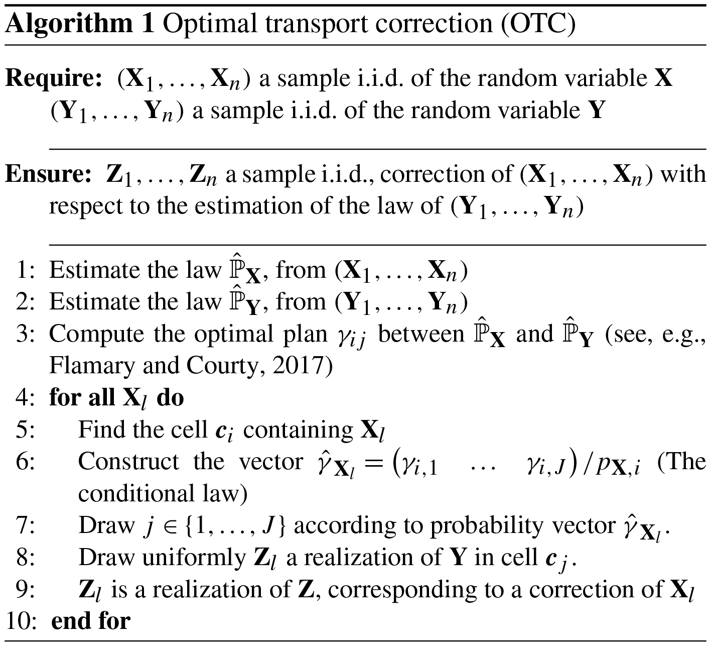
Finding γ_ij, i.e., solving the problem defined by constraints of Eqs. (2)–(3) and minimization of Eq. (4), is called a linear programming problem. It can be solved (for example) by the network simplex algorithm (see, e.g., Bazaraa et al., 2009). We use the python implementation of Flamary and Courty (2017). To correct X, we have to follow the plan of γ_ij. For a realization X_l of X, we take the cell c_i that contains X_l. Following $\widehat{\mathit{\gamma }}$, c_i is moved to c_j with probability ${\mathit{\gamma }}_{ij}/p_{\mathbf{X},i}$ (applying Eq. (2), the sum over j is 1). To determine c_j, we randomly draw it according to the conditional law ${\widehat{\mathit{\gamma }}}_{{\mathbf{X}}_l}=({\mathit{\gamma }}_{i\mathrm{1}},\mathrm{\dots },{\mathit{\gamma }}_{iJ})/p_{\mathbf{X},i}$. Finally, we draw uniformly y in c_j. This methodology is summarized in Algorithm A1, and we refer to it as optimal transport correction (OTC).

Note that the traditional one-dimensional quantile mapping preserves the ordering of quantiles. In the multivariate case, this type of property can be viewed as the Monge–Mather (1991) shortening principle (see, e.g., Villani, 2008, chap. 8). The idea is that the extremes of a multivariate distribution are moved to extremes, the boundary to the boundary, the level lines to level lines, etc.

Table 1Representation of bias correction in the context of climate change.

Download Print Version | Download XLSX

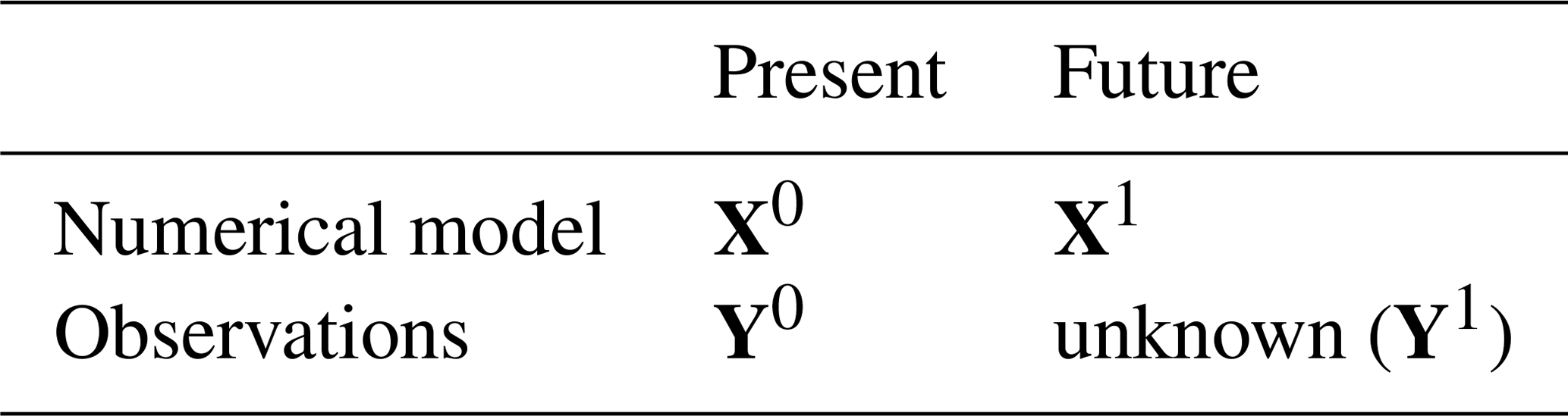
2.5 Non-stationary bias correction

Climate models offer a valuable tool to study future realistic climate trajectories. Climate model outputs of the present period need to be bias corrected with respect to current observations. Future climate simulations also need to be adjusted. However, no observation is available for the future and clear assumptions have to be made to correct simulations for future periods. Table 1 displays the basic framework of bias correction. Future unobserved data, say Y¹, should be inferred from the current reference vector, Y⁰, and two numerical runs, one in the present, say X⁰, and one in the future, say X¹. Period 0 is called the calibration period, and period 1 the projection period. In the univariate case, denoting Fⁱ (Gⁱ) the CDF of Xⁱ (Yⁱ), the CDF-t (CDF transform) method of Michelangeli et al. (2009) assumes that

Recombining Eq. (5), the CDF of Y¹ is given by $G^{\mathrm{1}}=G^{\mathrm{0}}\circ (F^{\mathrm{0}}{)}^{-\mathrm{1}}\circ F^{\mathrm{1}}$, and can be used to perform a quantile mapping correction. Here, the fundamental hypothesis ${\mathcal{T}}_{Y^{\mathrm{0}},Y^{\mathrm{1}}}={\mathcal{T}}_{X^{\mathrm{0}},X^{\mathrm{1}}}$ means that the transfer functions to capture the temporal changes are identical in the model and observational worlds.

CDF-t learns the change between X⁰ and X¹, and transfers it to Y⁰ to estimate Y¹. In the multivariate case, following CDF-t, we want to learn the evolution (i.e., the change or the temporal evolution) between X⁰ and X¹, and apply it to Y⁰. This generates Y¹, and OTC can then be applied between X¹ and Y¹. Note also that the reverse hypothesis ${\mathcal{T}}_{Y^{\mathrm{1}},X^{\mathrm{1}}}={\mathcal{T}}_{Y^{\mathrm{0}},X^{\mathrm{0}}}$ could be considered, meaning that the bias is learned, and transferred along the dynamic. In this case, the correction of example given in Sect. 3 does not correspond to the reference (not shown), so we rejected this assumption. Thus, our definition of non-stationary bias correction assumes a transfer of the evolution of the model to the observational world. Indeed, climate change is one of the main signals that we want to account for in the projected corrections. However, the change in the observations can be different, and therefore the resulting corrections can also be different from observations. Nevertheless, this methodology is justified because different simulations can have different evolutions; e.g., the four RCP scenarios provide four different simulations, giving four different corrections. This is also true for different climate models, which can show different changes. This information is therefore kept in the corrections.

Figure 2Estimation of the unobserved random variable Y¹. The random variables X⁰, X¹ and Y⁰ are known. Plans γ and φ are the optimal joint laws in the sense of Eqs. (2)–(4). $\stackrel{\mathrm{̃}}{\mathit{\phi }}$ is the evolution of Y⁰ estimated from γ and φ. OTC is used to correct X¹ with respect to the estimation of Y¹.

Download

Using OTC, we define two optimal plans: the optimal plan γ, between X⁰ and Y⁰, and the optimal plan φ, between X⁰ and X¹. The law γ is the bias between X⁰ and Y⁰, whereas φ is the evolution between X⁰ and X¹. Our goal is to move φ along γ, defining a plan $\stackrel{\mathrm{̃}}{\mathit{\phi }}$, to estimate Y¹ as the evolution of Y⁰, i.e., ${\mathbf{Y}}^{\mathrm{1}}=\stackrel{\mathrm{̃}}{\mathit{\phi }}\left({\mathbf{Y}}^{\mathrm{0}}\right)$. Then, we correct X¹ with respect to ${\mathbf{Y}}^{\mathrm{1}}=\stackrel{\mathrm{̃}}{\mathit{\phi }}\left({\mathbf{Y}}^{\mathrm{0}}\right)$, with the OTC method. This is summarized in Fig. 2.

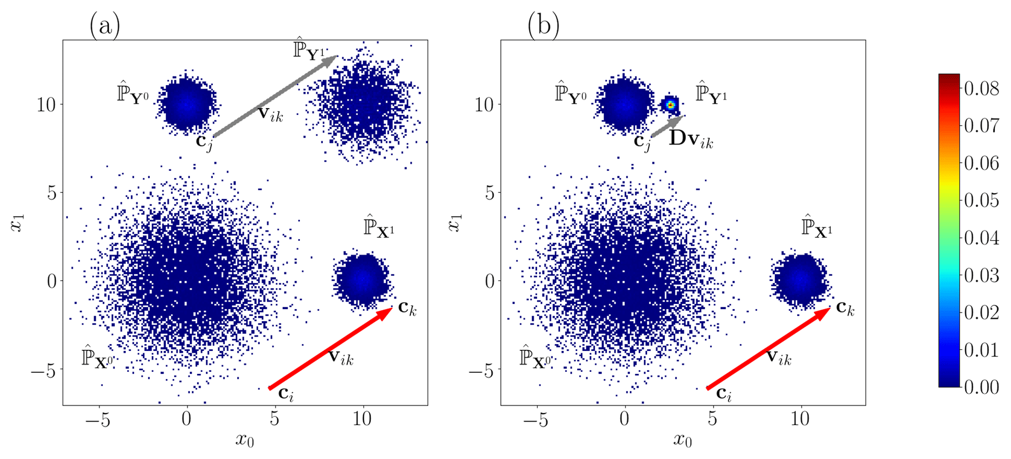
Figure 3Bivariate histogram with bin size equal to 0.1. In each panel we have a Gaussian law centered on (0,0) with covariance 4Id₂ (${\widehat{\mathbb{P}}}_{{\mathbf{X}}^{\mathrm{0}}}$), a Gaussian law centered on (10,0) with covariance 1∕4Id₂ (${\widehat{\mathbb{P}}}_{{\mathbf{X}}^{\mathrm{1}}}$) and a Gaussian law centered on (0,10) with covariance 1∕4Id₂ (${\widehat{\mathbb{P}}}_{{\mathbf{X}}^{\mathrm{1}}}$). The red arrow is the local evolution between ${\widehat{\mathbb{P}}}_{{\mathbf{X}}^{\mathrm{0}}}$ and ${\widehat{\mathbb{P}}}_{{\mathbf{X}}^{\mathrm{1}}}$. (a) The probability distribution ${\widehat{\mathbb{P}}}_{{\mathbf{Y}}^{\mathrm{1}}}$ is the correction with OTC-t and D=Id₂. The grey arrow is the estimation of the evolution of ${\widehat{\mathbb{P}}}_{{\mathbf{Y}}^{\mathrm{0}}}$. (b) The probability distribution ${\widehat{\mathbb{P}}}_{{\mathbf{Y}}^{\mathrm{1}}}$ is the correction with dOTC and D given by Eq. (6). The grey arrow is the estimation of the evolution of ${\widehat{\mathbb{P}}}_{{\mathbf{Y}}^{\mathrm{0}}}$.

Download

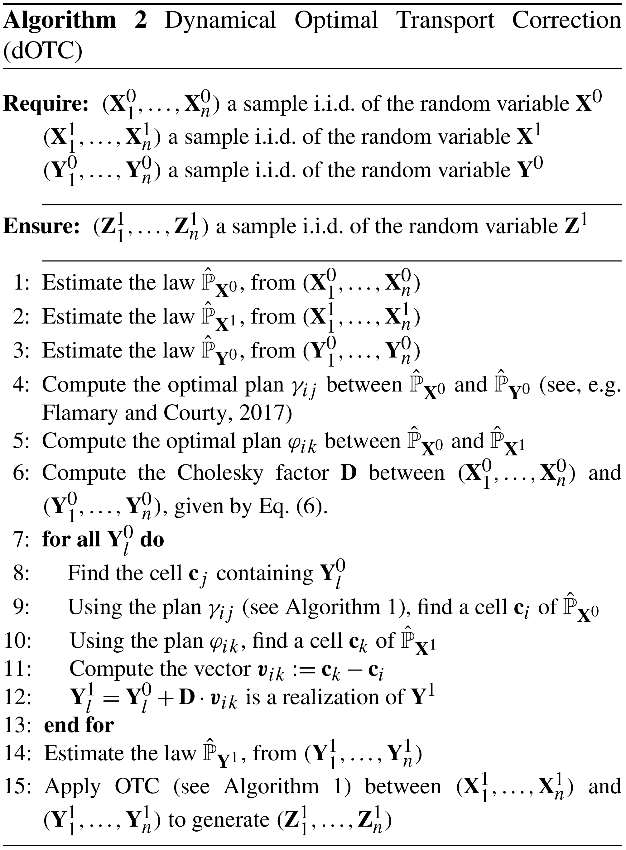
The estimation of $\stackrel{\mathrm{̃}}{\mathit{\phi }}$ is performed in three steps:

1. transformation of φ into a collection of vectors,

2. transferral of these vectors along γ and

3. adaptation of these vectors to Y⁰.

To illustrate our methodology, Fig. 3 shows an example where the random variables X⁰, X¹ and Y⁰ follow a bivariate Gaussian law. They are, respectively, centered at (0,0), (10,0) and (0,10), with covariance matrices 4×Id₂, Id₂∕4 and Id₂∕4 (the matrix Id_d is the d-dimensional identity matrix). Without loss of generality, we write the empirical distribution of X⁰, X¹ and Y⁰ as a sum of Dirac masses,

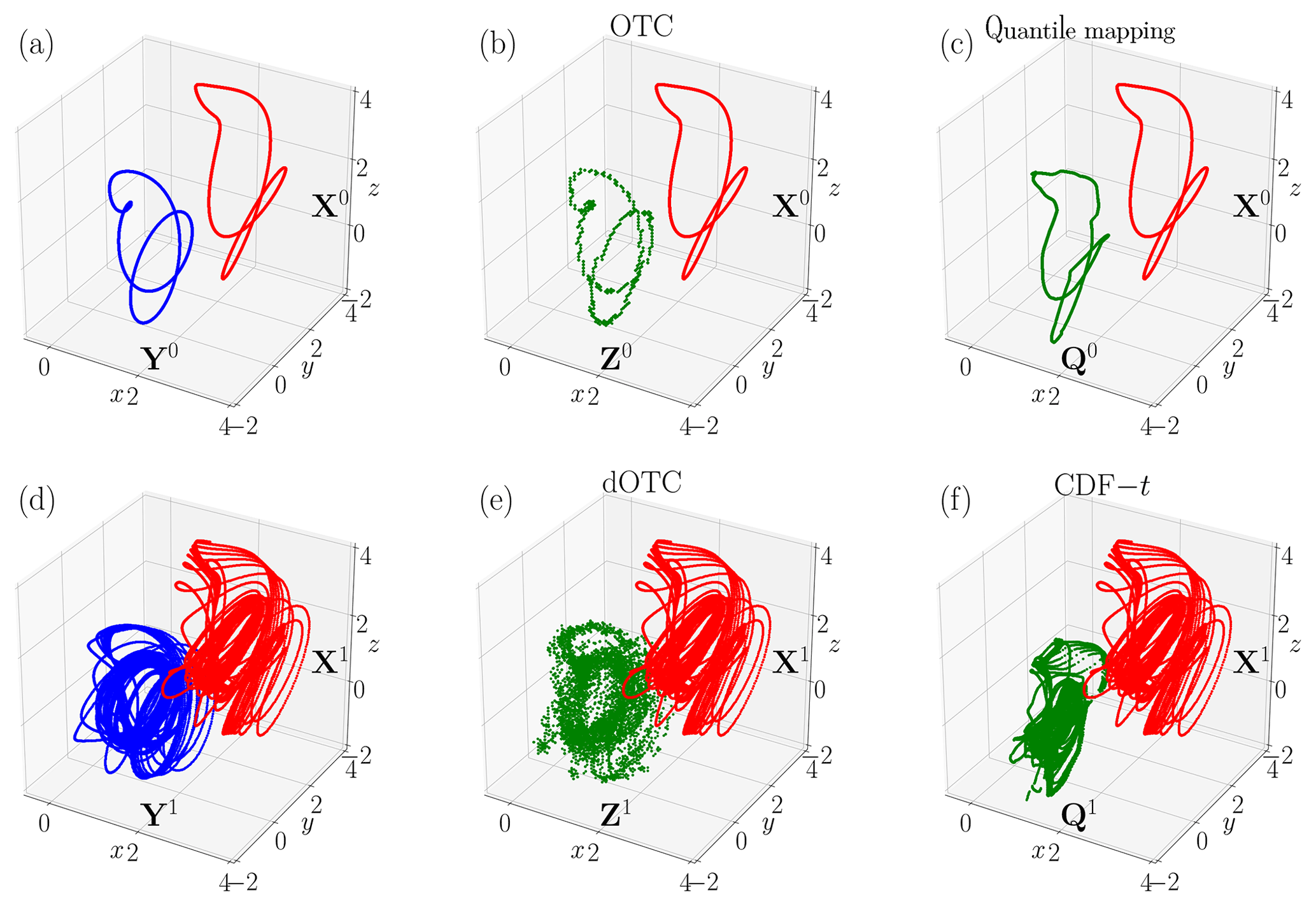
Figure 4Random variables generated by the Lorenz (1984) model, OTC, dOTC, quantile mapping and CDF-t. (a) Biased random variable X⁰ (red) and references Y⁰ (blue) for time period 0. (b) Biased random variable X⁰ (red) and correction Z⁰ with OTC (green). (c) Biased random variable X⁰ (red) and correction Q⁰ with quantile mapping (green). (d) Biased random variable X¹ (red) and references Y¹ (blue) for time period 1. (e) Biased random variable X¹ (red) and correction Z¹ with dOTC (green). (f) Biased random variable X¹ (red) and correction Q¹ with CDF-t (green).

Download

• Step 1. Transformation of φ. Using the OTC method, φ moves the bin c_i of ${\widehat{\mathbb{P}}}_{{\mathbf{X}}^{\mathrm{0}}}$ to the bin c_k of ${\widehat{\mathbb{P}}}_{{\mathbf{X}}^{\mathrm{1}}}$. The vector ${\mathit{v}}_{ik}:={\mathit{c}}_k-{\mathit{c}}_i$ represents the evolution from c_i to c_k (i.e., the local evolution between X⁰ and X¹). The collection of vectors v_ik is an estimation of the process between X⁰ and X¹. In Fig. 3, the red arrow is an example of vector v_ik.

• Step 2. Transfer along γ. Using the OTC method, γ moves the bin c_i of ${\widehat{\mathbb{P}}}_{{\mathbf{X}}^{\mathrm{0}}}$ to the bin c_j of ${\widehat{\mathbb{P}}}_{{\mathbf{Y}}^{\mathrm{0}}}$. Thus, the estimation of $\stackrel{\mathrm{̃}}{\mathit{\phi }}$ could be defined by the vector v_ik applied to c_j; i.e., a realization of Y¹ is given by c_j+v_ik. The grey arrow in Fig. 3a depicts this operation. But the v_ik can cross, and the correction is not coherent. This is due to normalizing issues and because the collection of vectors v_ik applied to Y⁰ does not define an optimal transport plan. The standard deviation decreases between X⁰ and X¹, whereas it increases between Y⁰ and Y¹ in our example. Furthermore, the quantiles are inverted in this example (low values are moved to high values). Consequently, we have to adapt the vectors v_ik to ${\widehat{\mathbb{P}}}_{{\mathbf{Y}}^{\mathrm{0}}}$.

• Step 3. Adaptation of v_ik. To solve this problem, we introduce a matrix factor D, which rescales the collection of vectors v_ik. In the univariate case, Bürger et al. (2011) proposed a factor ${\mathit{\sigma }}_{{\mathbf{Y}}^{\mathrm{0}}}{\mathit{\sigma }}_{{\mathbf{X}}^{\mathrm{0}}}^{-\mathrm{1}}$, where σ is the standard deviation. The idea is to remove the scale of X⁰ and to replace it by the scale of Y⁰. Bárdossy and Pegram (2012) and Cannon (2016) proposed a multivariate equivalent that uses the Cholesky decomposition of the covariance matrix. Denoting Σ the covariance matrix, and Cho(Σ) its Cholesky decomposition, we multiply (in a matrix sense) v_ik by the following matrix:

  $$\begin{array}{}\text{(6)}& \mathbf{D}:=\mathrm{Cho}\left({\mathrm{\Sigma }}_{{\mathbf{Y}}^{\mathrm{0}}}\right)\cdot \mathrm{Cho}({\mathrm{\Sigma }}_{{\mathbf{X}}^{\mathrm{0}}}{)}^{-\mathrm{1}}.\end{array}$$

  The Cholesky decomposition only exists if Σ is symmetric and positive-definite. Some covariance matrices do not have this property, e.g., highly correlated random variables. In such a case, Σ must be slightly perturbed to be positive-definite (see, e.g., Higham, 1988; Knol and ten Berge, 1989). Furthermore, the Cholesky decomposition can be poorly estimated if the number of available data is too small compared to the dimension. Indeed, the inverse of a covariance matrix is highly biased. In this case, a pragmatic solution is to replace the matrix D by the diagonal matrix of the standard deviation, i.e., $\mathbf{D}=\mathrm{diag}\left({\mathit{\sigma }}_{{\mathbf{Y}}^{\mathrm{0}}}{\mathit{\sigma }}_{{\mathbf{X}}^{\mathrm{0}}}^{-\mathrm{1}}\right)$.

Finally, a realization of Y¹ is given by ${\mathit{c}}_j+\mathbf{D}\cdot {\mathit{v}}_{ik}$. Figure 3b shows an estimation of Y¹. Visually, the shape of Y¹ appears coherent with the evolution between X⁰ and X¹. The mean of Y¹ is (2.53,10). The standard deviation between X⁰ and X¹ is divided by 4. The mean shift between X⁰ and X¹ is (10,0). This shift of 10 units is correctly taken into account in the rescaling of Y⁰ by the standard deviation (equal to 4) between X⁰ and X¹:

The value of the covariance matrix of Y¹ is ${\mathrm{\Sigma }}_{{\mathbf{Y}}^{\mathrm{1}}}\simeq \mathrm{0.018}\times {\mathbf{Id}}_{\mathrm{2}}$. It is close to the expected value $(\mathrm{1}/\mathrm{4})/\mathrm{16}\times {\mathbf{Id}}_{\mathrm{2}}\simeq \mathrm{0.015}\times {\mathbf{Id}}_{\mathrm{2}}$. The shift of 10 units of the model is not followed. It is interpreted as a correction of the bias into the evolution of the model. However, depending on the hypotheses desired by the user, the dOTC method can easily provide corrections whose mean evolutions and trends are in agreement with those given by the simulations to be corrected, like in the EDQM bias correction method (Li et al., 2010). The complete method of correction is summarized in Algorithm A2. We refer to it as dOTC (dynamical optimal transport correction).

We first propose evaluating OTC and dOTC on an idealized case.

3.1 Model and methodology

To evaluate our bias correction method, we construct an idealized biased case, based on the Lorenz (1984) model. This three-dimensional system is generated by the differential equations

The function ψ(t) is a linear forcing proposed by Drótos et al. (2015). Classically, ψ also contains a seasonal cycle (Lorenz, 1990), where the length of a “year” is fixed at t=73 time units. Here we integrate this equation for the following forcing between 0 and 7×73 (i.e., 7 “years” of integration):

The integration is performed with a Runge–Kutta (order 4) scheme with a time step of size 0.005. All trajectories of the Lorenz (1984) model converge on a unique subset of ℝ³ (called an attractor), and remain trapped on it. According to Drótos et al. (2015), the first 5 “years” correspond to the time required to trap the trajectories.

One realization of random variable Y⁰ (Y¹) is year 6 (year 7). Each year contains $\mathrm{14}\mathrm{600}(=\mathrm{73}/\mathrm{0.005})$ elements. According to Eq. (8), the linear forcing is applied during year 7. The non-stationarity is induced by the change between the two time periods.

We introduce a bias by multiplying each point of the trajectories by a triangular matrix S, and add a vector m, i.e., $\mathbf{X}=\mathbf{SY}+\mathit{m}$. The addition changes the mean, whereas the multiplication alters the covariances. The matrix S is chosen empirically such that the covariance matrices of X⁰, X¹, Y⁰ and Y¹ differ. We fix

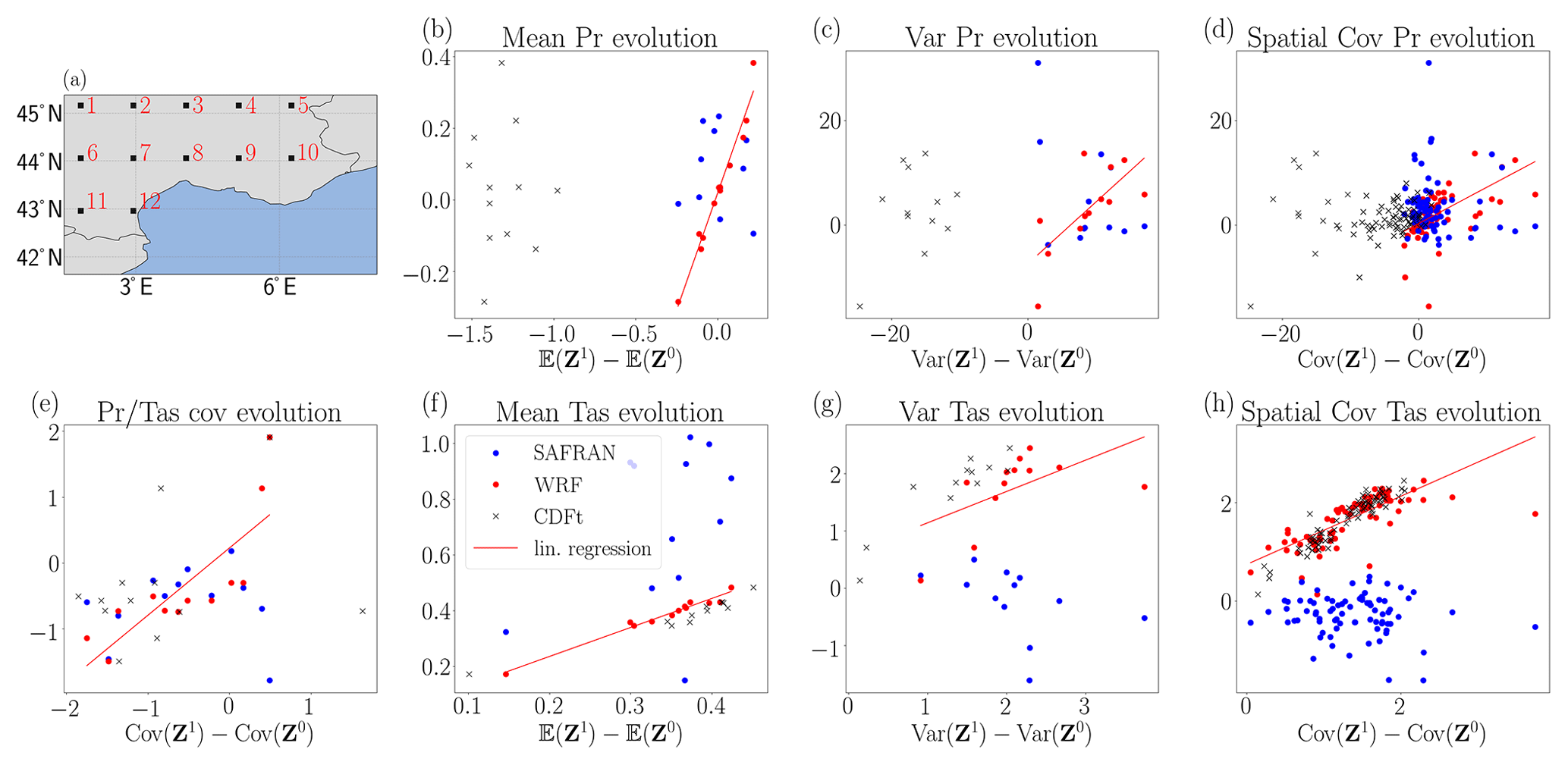
Figure 5(a) Map of the southeast of France. The 12 black squares are the locations where corrections are performed. (b–h) The x axis of the panels is the evolution of the correction with dOTC. The y axis of panels (b)–(h) is the evolution of WRF in red and the evolution of SAFRAN in blue. The red line is the linear regression between the evolution of correction and the evolution of WRF. The black cross markers are the scatterplots between the evolution of correction with CDF-t and evolution of WRF. (b) Evolution of mean precipitation, i.e., difference between the projection period and the calibration period. (c) Evolution of variance of precipitation. (d) Evolution of spatial covariance of precipitation. (e) Evolution of covariance between precipitation and temperatures. (f) Evolution of mean temperatures. (g) Evolution of variance of temperatures. (h) Evolution of spatial covariance of temperatures.

Download

The random variables X and Y are plotted in Fig. 4a, d. The blue (red) curve of Fig. 4a is the trajectory of Y⁰ (X⁰). The mean is largely altered. We estimate the covariance matrices as

Similarly to Fig. 4a, d depicts in blue Y¹ and in red X¹. The forcing of Eq. (8) has changed the properties of the trajectories, and they became chaotic. It is worthwhile noticing that the dynamic of Y is comparable to the one of X. The covariance matrices are largely affected:

We estimate the empirical distributions ${\mathbb{P}}_{{\mathbf{Y}}^{\mathrm{0}}}$, ${\mathbb{P}}_{{\mathbf{Y}}^{\mathrm{1}}}$, ${\mathbb{P}}_{{\mathbf{X}}^{\mathrm{0}}}$ and ${\mathbb{P}}_{{\mathbf{X}}^{\mathrm{1}}}$ with a three-dimensional histogram. We cut a large cube around the trajectories into cells of size $\mathrm{0.2}\times \mathrm{0.2}\times \mathrm{0.2}$. Then we count the number of points in each cell.

Finally, we evaluate the quality of the correction by comparing the covariance matrices of Y⁰ and X⁰, and the covariance matrices of Y¹ and X¹.

3.2 Correction of the biased Lorenz (1984) model

We apply our method to correct X⁰ and X¹. The random variable X⁰ is corrected with respect to Y⁰ and using the OTC method. The random variable X¹ is corrected with respect to the estimation of Y¹, coming from the dOTC method. The resulting random variables Z⁰ and Z¹ are given in Fig. 4b, e. We show in Fig. 4c, f a univariate correction with quantile mapping for the period 0, generating the random variable Q⁰. The same is shown for CDFt, period 1 and the random variable Q¹.

The correction Z⁰ is visually very similar to the reference in blue in Fig. 4a. The covariance matrix is almost perfectly reproduced:

The correction Z¹ is depicted in green in Fig. 4d. It is visually hard to compare to Fig. 4b, but we recognize Y¹. The covariance matrix is correctly rectified:

Finally, the cost of transformation, given by Eq. (1), of Z¹ into Y¹ is 93 % smaller than the cost between Y¹ and X¹; i.e., ${\mathbb{P}}_{{\mathbf{Z}}^{\mathrm{1}}}$ is more similar to ${\mathbb{P}}_{{\mathbf{Y}}^{\mathrm{1}}}$ than ${\mathbb{P}}_{{\mathbf{X}}^{\mathrm{1}}}$. Furthermore, if we replace the Cholesky matrix of dOTC by the matrix of standard deviation, the maximum difference between covariance matrices increases to 0.22, but the cost is 85 % smaller. Thus, using the standard deviation slightly degrades the correction. However, visually, it is very hard to distinguish the corrections with the Cholesky matrix or the standard deviation matrix. The figure corresponding to Fig. 4 with the standard deviation matrix is given in the Supplement.

By contrast, Q⁰ and Q¹, depicted, respectively, in Fig. 4c, f, do not reproduce Y⁰ and Y¹. Thus, the multivariate correction is largely better than the univariate correction. This is confirmed by the covariance matrices, which reproduce exactly the covariances of X⁰ and X¹:

We have performed a tri-variate correction on a nonlinear system exhibiting non-standard probability measures (i.e., non-Gaussian, non-exponential). In the stationary case, the OTC method works almost perfectly. In the non-stationary case, the dOTC method produces a probability distribution closed to the expected result. We propose now to apply OTC and dOTC to climate model simulations.

4.1 Data

The dataset used as a reference for the bias correction (BC) is the Systeme d'Analyse Fournissant des Renseignements Atmospheriques a la Neige (SAFRAN, Vidal et al., 2010) reanalysis. SAFRAN is a hourly reanalysis over France between 1958 and present, with a horizontal resolution of 8 km × 8 km. Quintana-Seguí et al. (2008) claimed that the daily mean of the surface atmospheric temperature (tas) and precipitation (pr) presents no bias compared to observations from the climatological database of Météo-France. This justifies the use of SAFRAN as a reference.

We test our multivariate BC method on a simulation of the Weather Research and Forecast (WRF) atmospheric model (Skamarock et al., 2008) performed within the EURO-CORDEX initiative (Vautard et al., 2013; Jacob et al., 2014) with a 0.11^∘ × 0.11^∘ horizontal resolution. The boundaries of the simulation were forced by a historical simulation of the Institut Pierre-Simon Laplace (IPSL) coupled model (Marti et al., 2010; Dufresne et al., 2013). This EURO-CORDEX historical simulation will be called “WRF” in the following.

SAFRAN and WRF data are re-mapped onto the same grid, with a spatial resolution of 0.11^∘ × 0.11^∘ (i.e., ∼ 12 km × 12 km). The nearest neighbor interpolation is used. We only keep the land region comprised in 1.8–7.85^∘ E × 41.8–45.2^∘ N, i.e., covering the southeast of France. This region is characterized by a complex topography, which creates a strong spatial heterogeneity, especially for precipitation. For the present application, we extract 12 grid points regularly spaced (see Fig. 5a), with a one-to-one spatial correspondence between SAFRAN and WRF.

In both datasets, we will consider daily surface air temperatures and precipitation. The goal of this section is to correct the bias in tas and pr in the WRF data with respect to SAFRAN.

4.2 Cross-validation protocol

We focus on the daily timescale over the 1970–2000 period. We correct the warm season (May–September). The analysis and conclusions are available for the cold season, and the corresponding figure (i.e., Fig. 5) is given in the Supplement. We split that period into two sub-periods, 1970–1985 (2295 days) and 1985–2000 (2295 days), to perform a cross-validation. The SAFRAN (WRF) values over the first time period correspond to the random variable Y⁰ (X⁰), and are called the calibration period. The SAFRAN (WRF) values over the second time period correspond to Y¹ (X¹), and are called the projection period. SAFRAN during 1985–2000 (i.e., Y¹) is assumed to be unknown, and is used for cross-validation.

We perform two bias corrections: univariate and 24-variate (12 grid points and 2 variables).

1. For univariate correction, quantile mapping is used for the calibration period, and CDF-t for the projection period.

2. For 24-variate correction, OTC is used for the calibration period, and dOTC for the projection period. The spatial structure and the dependence between the two variables are used. Due to the dimension, the Cholesky matrix is poorly estimated. We replace it by the matrix of standard deviation in the rescaling step.

We estimate the empirical distributions by computing histograms with bins of size 0.1 in each dimension. Furthermore, CDF-t and dOTC can shift close to 0 values to negative values for precipitation. Thus, negative precipitation values are replaced by 0 after correction. We test the quality of the correction by plotting the evolution of the mean, the standard deviation, and the spatial and inter-variable covariance, i.e., the difference between the projection and calibration periods. These indicators are summarized in Fig. 5. During the calibration period, the goal is that the probability distribution of correction of the WRF simulation will be the probability distribution of SAFRAN. By construction of OTC, the correction is almost perfect, and we focus on the projection period. In the projection period, the goal is that the evolution of corrections will be close to the evolution of the WRF simulation.

4.3 Evolution analysis

As we have seen in the previous section, the corrections of X¹ and Y¹ are identical only if the evolution of SAFRAN is identical to the evolution of WRF. To analyze the evolution of WRF, SAFRAN and the corrections, we compute the difference of statistical indicators between the projection and the calibration period at each grid point. The indicators are the mean (Fig. 5b, f), the variance (Fig. 5c, g), the covariance between pr and tas (Fig. 5e) and the spatial covariance for each variable (Fig. 5d, h).

Table 2r-value, p-value and standard error (SE) of linear regression between the evolution of correction and evolution of WRF.

Download Print Version | Download XLSX

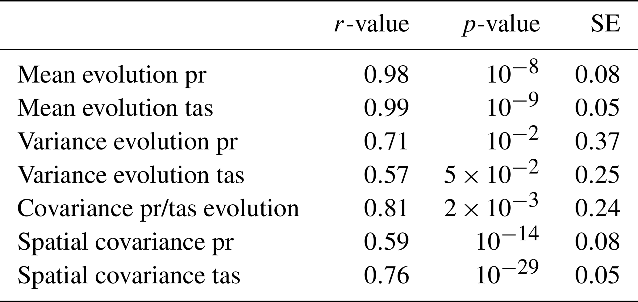
The x axis of Fig. 5a–h is the evolution of the correction (i.e., 𝔼(Z¹)−𝔼(Z⁰),…). The y axis of Fig. 5a–h is the evolution of WRF in red (i.e., 𝔼(X¹)−𝔼(X⁰),…), and the evolution of SAFRAN in blue (i.e., 𝔼(Y¹)−𝔼(Y⁰),…). Furthermore, the red line is the linear regression between the evolution of the 24-variate correction and the evolution of WRF. The correlation (r-value), p-value and standard error of each linear regression are summarized in Table 2.

The linear regression between evolution of 24-variate correction and evolution of WRF (red line) shows a strong statistical link for all statistical indicators. The evolution of the mean is almost perfectly reproduced for the two variables (r-values is at least equal to 0.98, with a maximal p-value at 10⁻⁹). The evolution of variance of WRF is also reproduced, the linear regression being significant (maximal p-value is $\mathrm{5}\times {\mathrm{10}}^{-\mathrm{2}}$).

The evolution of dependence structure is given by the evolution of spatial and inter-variables covariance. The minimal r-value for linear regression is equal to 0.59 with a maximal p-value equal to $\mathrm{2}\times {\mathrm{10}}^{-\mathrm{3}}$. This means that dOTC reproduces the evolution of WRF between calibration and projection period. Because the calibration period is perfectly corrected, the correction during projection period appears as the evolution of WRF, applied to SAFRAN.

A linear regression, the Spearman rank correlation between the evolution of SAFRAN, and the evolution of the correction with WRF do not show a significant statistical link (not shown). We conclude that the evolution of WRF is different of the evolution of SAFRAN. This indicates it is not possible to reproduce SAFRAN during projection period using dOTC and WRF. For example, WRF predicts an increase between 0.2 and 0.4 K of the mean temperature, whereas SAFRAN gives an increase between 0.2 and 1 K.

The correction with CDF-t appears to be satisfactory for the temperatures, and very similar to the correction with dOTC. But for the precipitation, the structure is not coherent with WRF or SAFRAN. This dissimilarity is due to the difference between the probability distribution of temperatures (quasi-Gaussian) and precipitations (exponential/Gamma laws).

We conclude that the evolution of the 24-variate correction with dOTC between calibration and projection periods is close to the evolution of WRF. Furthermore, the evolution of SAFRAN is very different from the evolution of WRF. In particular, this example illustrates how the classical cross-validation methodology does not differentiate the variations of SAFRAN and WRF, and that the correction can not be compared to the reference during the projection period.