the Creative Commons Attribution 4.0 License.
the Creative Commons Attribution 4.0 License.
 | 13 Feb 2019
A simple topography-driven and calibration-free runoff generation module
Christian Birkel
Markus Hrachowitz
Doerthe Tetzlaff
Chris Soulsby
Hubert H. G. Savenije
Reading landscapes and developing calibration-free runoff generation models that adequately reflect land surface heterogeneities remains the focus of much hydrological research. In this study, we report a novel and simple topography-driven runoff generation parameterization – the HAND-based Storage Capacity curve (HSC), which uses a topographic index (HAND, Height Above the Nearest Drainage) to identify hydrological similarity and the extent of saturated areas in catchments. The HSC can be used as a module in any conceptual rainfall–runoff model. Further, coupling the HSC parameterization with the mass curve technique (MCT) to estimate root zone storage capacity (SuMax), we developed a calibration-free runoff generation module, HSC-MCT. The runoff generation modules of HBV and TOPMODEL were used for comparison purposes. The performance of these two modules (HSC and HSC-MCT) was first checked against the data-rich Bruntland Burn (BB) catchment in Scotland, which has a long time series of field-mapped saturation area extent. We found that HSC, HBV and TOPMODEL all perform well to reproduce the hydrograph, but the HSC module performs better in reproducing saturated area variation, in terms of correlation coefficient and spatial pattern. The HSC and HSC-MCT modules were subsequently tested for 323 MOPEX catchments in the US, with diverse climate, soil, vegetation and geological characteristics. In comparison with HBV and TOPMODEL, the HSC performs better in both calibration and validation, particularly in the catchments with gentle topography, less forest cover, and arid climate. Despite having no calibrated parameters, the HSC-MCT module performed comparably well with calibrated modules, highlighting the robustness of the HSC parameterization to describe the spatial distribution of the root zone storage capacity and the efficiency of the MCT method to estimate SuMax. This novel and calibration-free runoff generation module helps to improve the prediction in ungauged basins and has great potential to be generalized at the global scale.
- Article
(7897 KB) -
Supplement
(606 KB) - BibTeX
- EndNote


Determining the volume and timing of runoff generation from rainfall inputs remains a central challenge in rainfall–runoff modeling (Beven, 2012; McDonnell, 2013). Creating a simple, calibration-free, but robust runoff generation module has been, and continues to be, an essential pursuit of hydrological modelers. Although we have made tremendous advances in enhancing our ability in prediction in ungauged basins (PUB) (Sivapalan et al., 2003; Blöschl et al., 2013; Hrachowitz et al., 2013), it is not uncommon that models become increasingly complicated in order to capture the details of hydrological processes shown by empirical studies (McDonnell, 2007; Sivapalan, 2009; Yu et al., 2014). More detailed process conceptualization normally demands higher data requirements than our standard climatological and hydrological networks can provide, leading to more calibrated parameters and a probable increase in model uncertainty (Sivapalan, 2009).
Hydrological connectivity is a key characteristic of catchment functioning, controlling runoff generation. It is a property emerging at larger scales, describing the temporal dynamics of how spatially heterogeneous storage thresholds in different parts of catchments are exceeded to contribute to storm runoff generation and how they are thus “connected to the stream” (e.g., Zehe and Blöschl, 2004; Bracken and Croke, 2007; Zehe and Sivapalan, 2009; Ali et al., 2014; Blume and van Meerveld, 2015). Connectivity is controlled by a multitude of factors (Ali and Roy, 2010), including but not limited to surface (e.g., Jencso et al., 2009) and subsurface topography (e.g., Tromp-van Meerveld and McDonnell, 2006), soils (including preferential flow networks; e.g., Zehe et al., 2006; Weiler and McDonnell, 2007), land cover (e.g., Imeson and Prinsen, 2004; Jencso and McGlynn, 2011), and the wetness state of the system (e.g., Detty and McGuire, 2010; Penna et al., 2011; McMillan et al., 2014; Nippgen et al., 2015).
In detailed distributed hydrological bottom-up models, connectivity emerges from the interplay of topography, soil type, and water table depth. For example, TOPMODEL (Beven and Kirkby, 1979; Beven and Freer, 2001) uses the topographic wetness index (TWI) to distinguish hydrologic similarity; and SHE (Abbott et al., 1986) and tRIBS (Ivanov et al., 2004; Vivoni et al., 2005) use partial differential equations to describe the water movement based on pressure gradients obtained by topography; and the representative elementary watershed (REW) approach divides catchments into a number of REWs to build balance and constitutive equations for hydrological simulation (Reggiani et al., 1999; Zhang and Savenije, 2005; Tian et al., 2008). As the relevant model parameters such as local topographic slope and hydraulic conductivity can, in spite of several unresolved issues for example relating to the differences in the observation and modeling scales (e.g., Beven, 1989; Zehe et al., 2014), be obtained from direct observations, they could in principle be applied without calibration.
Zooming out to the macro-scale, top-down models, in contrast, are based on emergent functional relationships that integrate system-internal heterogeneity (Sivapalan, 2005). These functional relationships require parameters that are effective on the modeling scale and that can largely not be directly determined with small-scale field observations (cf. Beven, 1995) and thus traditionally determined by calibration. However, frequently the number of observed variables for model calibration is, if available at all, limited to time series of streamflow. The absence of more variables to constrain models results in such models being ill-posed inverse problems. Equifinality in parameterization and in the choice of parameters then results in considerable model uncertainty (e.g., Beven, 1993, 2006). To limit this problem and to also allow predictions in the vast majority of ungauged catchments, it is therefore desirable to find ways to directly infer effective model parameters at the modeling scale from readily available data (Hrachowitz et al., 2013).
The component that is central for establishing connectivity in most top-down models is the soil moisture routine. Briefly, it controls the dynamics of water storage and release in the unsaturated root zone and partitions water into evaporative fluxes, groundwater recharge, and fast lateral storm flow generating runoff (Gao et al., 2018a; Shao et al., 2018), the latter of which is critical from the aspect of connectivity. In the majority of regions, Hortonian overland flow (HOF, i.e., infiltration excess overland flow) is of minor importance (Dunne and Black, 1970; Sklash and Farvolden, 1979; Beven, 2004; Burt and McDonnell, 2015), even in arid regions where often most locally generated HOF is re-infiltrated while flowing on hillslopes (Liu et al., 2012; Zhao et al., 2019) and never reaches the stream channel network. Thus the term saturation excess flow (SEF) can represent, depending on the model and the area of application, different processes, such as saturation overland flow, preferential flow, flow through shallow, high-permeability soil layers, or combinations thereof. The interplay between water volumes that are stored and those that are released laterally to the stream via fast, connected flow paths (“connectivity”) is in most top-down models described by functions between water stored in the unsaturated root zone (“soil moisture”) and the areal proportion of heterogeneous, local storage thresholds that are exceeded and thus “connected” (Zhao et al., 1980). In other words, in those parts of a catchment where the storage threshold is exceeded it will generate lateral flows, and can alternatively be interpreted as a runoff coefficient (e.g., Ponce and Hawkins, 1996; Perrin and Andreassian, 2001; Fenicia et al., 2007; Bergström and Lindström, 2015). Thus the idea goes back to the variable contributing area concept, assuming that only partial areas of a catchment, where soils are saturated and thus storage thresholds are exceeded, contribute to runoff (Hewlett, 1961; Dunne and Black, 1970; Hewlett and Troendle, 1975). Although originally developed for catchments dominated by saturation overland flow, the extension of the concept to subsurface connectivity, illustrating that surface and subsurface connectivity are “two sides of the same coin” (McDonnell, 2013), proved highly valuable for models such as Xinanjiang (Zhao et al., 1980), HBV (Bergström and Forsman, 1973; Bergström and Lindström, 2015), SCS-CN (Ponce and Hawkins, 1996; Bartlett et al., 2016), FLEX (Fenicia et al., 2008), and GR4J (Perrin and Andreassian et al., 2001).
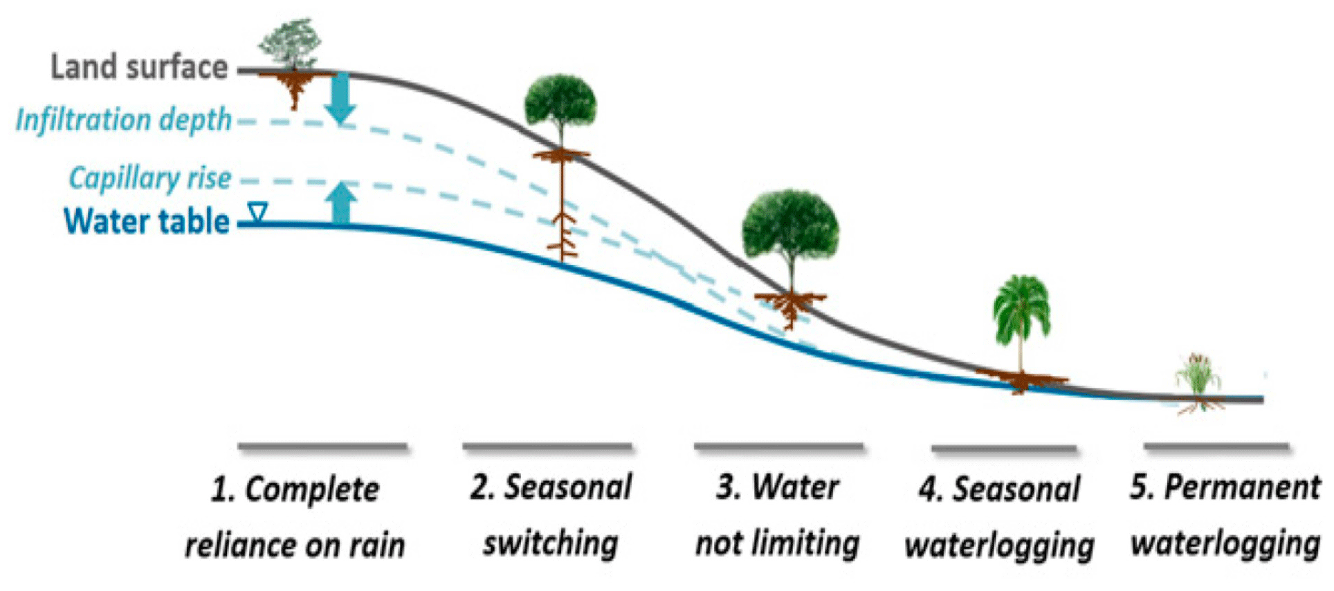
Figure 1The variation of plant rooting depths along a hillslope profile, showing the impact of HAND (Height Above the Nearest Drainage) on rooting depth (Taken from Fan et al., 2017 by permission of PNAS).
Among these models, connectivity is formulated in a general form as , where CR is the runoff coefficient; i.e., the proportion of the catchment generating runoff, SU(t), is the catchment water content in the unsaturated root zone at any time t, SuMax is a parameter representing the total storage capacity in the unsaturated root zone, and β is a shape parameter, representing the spatial distribution of heterogeneous storage capacities in the unsaturated root zone. The parameters of these functions are typically calibrated. In spite of being the core component of soil moisture routines in many top-down models, little effort was previously invested to find ways to determine the parameters at the catchment scale directly from available data. An important step towards understanding and quantifying connectivity patterns directly based on observations was recently achieved by intensive experimental work in the Tenderfoot Creek catchments in Montana, US. In their work, Jencso et al. (2009) were able to show that connectivity of individual hillslopes in their headwater catchments is highly related to their respective upslope accumulated areas. Using this close relationship, Smith et al. (2013) successfully developed a simple top-down model with very limited need for calibration, emphasizing the value of “enforcing field-based limits on model parameters” (Smith et al., 2016). Based on hydrological landscape analysis, the FLEX-Topo model (Savenije, 2010) can dramatically reduce the need for calibration (Gharari et al., 2014), and holds considerable potential for spatial model transferability without the need for parameter re-calibration (Gao et al., 2014a; H. Gao et al., 2016). In a recent development, several studies suggest that SuMax can be robustly and directly inferred from long-term water balance data by the mass curve technique (MCT) (Gao et al., 2014a; de Boer-Euser et al., 2016; Nijzink et al., 2016). The MCT is an engineering method for reservoir design, in which the reservoir size is estimated as a function of accumulated inflow and human water demand. The MCT treats the root zone as a reservoir, and estimates catchment-scale SuMax from measurable hydrometeorological data, without the need for further calibration. This leaves shape parameter β as the only free calibration parameter for soil moisture routines of that form. Topography is often the dominant driver of water movement caused by prevailing hydraulic gradients. More crucially, topography usually provides an integrating indicator for hydrological behavior, since topography is usually closely related to other landscape elements, such as soil vegetation climate and even geology (Seibert et al., 2007; Savenije, 2010; Rempe and Dietrich, 2014; Gao et al., 2014b; Maxwell and Condon, 2016; Gomes, 2016). The Height Above the Nearest Drainage (HAND; Rennó et al., 2008; Nobre et al., 2011; Gharari et al., 2011), which can be computed from readily available digital elevation models (DEMs), could potentially provide first-order estimates of groundwater depth, as there is some experimental evidence that with increasing HAND, groundwater depths similarly increase (e.g., Haria and Shand, 2004; Molenat et al., 2005, 2008; Shand et al., 2005; Condon and Maxwell, 2015; Maxwell and Condon, 2016). HAND can be interpreted as a proxy of the hydraulic head and is thus potentially more hydrologically informative than the topographic elevation above sea level (Nobre et al., 2011). Compared with the TWI in TOPMODEL, HAND is an explicit measure of a physical feature linking terrain to water-related potential energy for local drainage (Nobre et al., 2011). More interestingly, topographic structure emerges as a powerful force determining rooting depth under a given climate or within a biome (Fig. 1), revealed by a global synthesis of 2200 root observations of >1000 species (Fan et al., 2017). This leads us to think from an ecological perspective to use the topographic information as an indicator of root zone spatial distribution without calibrating the β, and coupling it with the MCT method to estimate the SuMax, to eventually create a calibration-free runoff generation module.
In this study we are therefore going to test the hypotheses that (1) HAND can be linked to the spatial distribution of storage capacities and therefore can be used to develop a new runoff generation module (HAND-based Storage Capacity curve, i.e., HSC); (2) the distribution of storage capacities determined by HAND contains different information than the topographic wetness index; (3) the HSC together with water balance-based estimates of SuMax (MCT method) allow the formulation of calibration-free parameterizations of soil moisture routines in top-down models directly based on observations. All these hypotheses will be tested firstly in a small data-rich experimental catchment (the Bruntland Burn catchment in Scotland), and then apply the model to a wide range of larger MOPEX catchments (Model Parameter Estimation Experiment).
This paper is structured as follows. In Sect. 2, we describe two of our proposed modules, i.e., HSC and HSC-MCT, and two benchmark models (HBV, TOPMODEL). This section also includes the description of other modules (i.e., interception, evaporation, and routing) in rainfall–runoff modeling, and the methods for model evaluation, calibration, and validation. Section 3 reviews the empirically based knowledge of the Bruntland Burn catchment in Scotland and the hydrometeorological and topographic datasets of MOPEX catchments in the US for model comparison. Sections 4 and 5 present the model comparison results. Section 6 interprets the relation between rainfall–runoff processes and topography, catchment heterogeneity, and simple models, and the implications and limitations of our proposed modules. The conclusions are briefly reviewed in Sect. 7.
Based on our perceptual model that saturation excess flow (SEF) is the dominant runoff generation mechanism in most cases, we developed the HAND-based Storage Capacity curve (HSC) module. Subsequently, estimating the parameter of root zone storage capacity (SuMax) by the MCT method without calibration, the HSC-MCT was developed. In order to assess the performance of our proposed modules, two widely used runoff generation modules, i.e., the HBV power function and TOPMODEL module, were set as benchmarks. Other modules, i.e., interception, evaporation, and routing, are kept with identical structure and parameterization for the four rainfall–runoff models (HBV, TOPMODEL, HSC, and HSC-MCT, whose names are from their runoff generation modules), to independently diagnose the difference among runoff generation modules (Clark et al., 2008, 2011).
2.1 Two benchmark modules
HBV power function
The HBV runoff generation module applies an empirical power function to estimate the nonlinear relationship between the runoff coefficient and soil moisture (Bergström and Forsman, 1973; Bergström and Lindström, 2015). The function is written as
where As (–) represents the contributing area, which equals the runoff coefficient of a certain rainfall event; Su (mm) represents the averaged root zone soil moisture; SuMax (mm) is the averaged root zone storage capacity of the studied catchment; β (–) is the parameter determining the shape of the power function. The prior range of β can be from 0.1 to 5. The Su and As have a linear relation, while β equals 1. And the shape becomes convex while the β is less than 1, and the shape turns to concave while the β is larger than 1. In most situations, SuMax and β are two free parameters, cannot be directly measured at the catchment scale, and need to be calibrated based on observed rainfall–runoff data.
TOPMODEL module
The TOPMODEL assumes topographic information captures the runoff generation heterogeneity at the catchment scale, and the TWI is used as an index to identify rainfall–runoff similarity (Beven and Kirkby, 1979; Sivapalan et al., 1997). Areas with similar TWI values are regarded as possessing equal runoff generation potential. More specifically, the areas with larger TWI values tend to be saturated first and contribute to SEF; but the areas with lower TWI values need more water to reach saturation and generate runoff. The equations are written as follow:
where Di (mm) is the local storage deficit below saturation at a specific location (i); (mm) is the averaged water deficit of the entire catchment (Eq. 2), which equals (SuMax−Su), as shown in Eq. (3). ITW_i is the local ITW value. is the averaged TWI of the entire catchment. Equation (2) means in a certain soil moisture deficit condition for the entire catchment (), the soil moisture deficit of a specific location (Di), is determined by the catchment topography (ITW and ITW_i), and the root zone storage capacity (SuMax). Therefore, the areas with Di less than zero are the saturated areas (As_i), equal to the contributing areas. The integration of the As_i areas (As), as presented in Eq. (4), is the runoff contributing area, which equals the runoff coefficient of that rainfall event.
Besides continuous rainfall–runoff calculation, Eqs. (2)–(4) also allow us to obtain the contributing area (As) from the estimated relative soil moisture (Su∕SuMax) and then map it back to the original TWI map, which makes it possible to test the simulated contributing area by field measurement. It is worth mentioning that the TOPMODEL in this study is a simplified version, and not identical to the original one, which combines the saturated and unsaturated soil components.
2.2 HSC module
In the HSC module, we assume (1) primarily saturation excess flow as the dominant runoff generation mechanism; (2) the local root zone storage capacity has a positive and linear relationship with HAND, from which we can derive the spatial distribution of the root zone storage capacity; (3) rainfall firstly feeds local soil moisture deficit, and no runoff can be generated before local soil moisture being saturated.
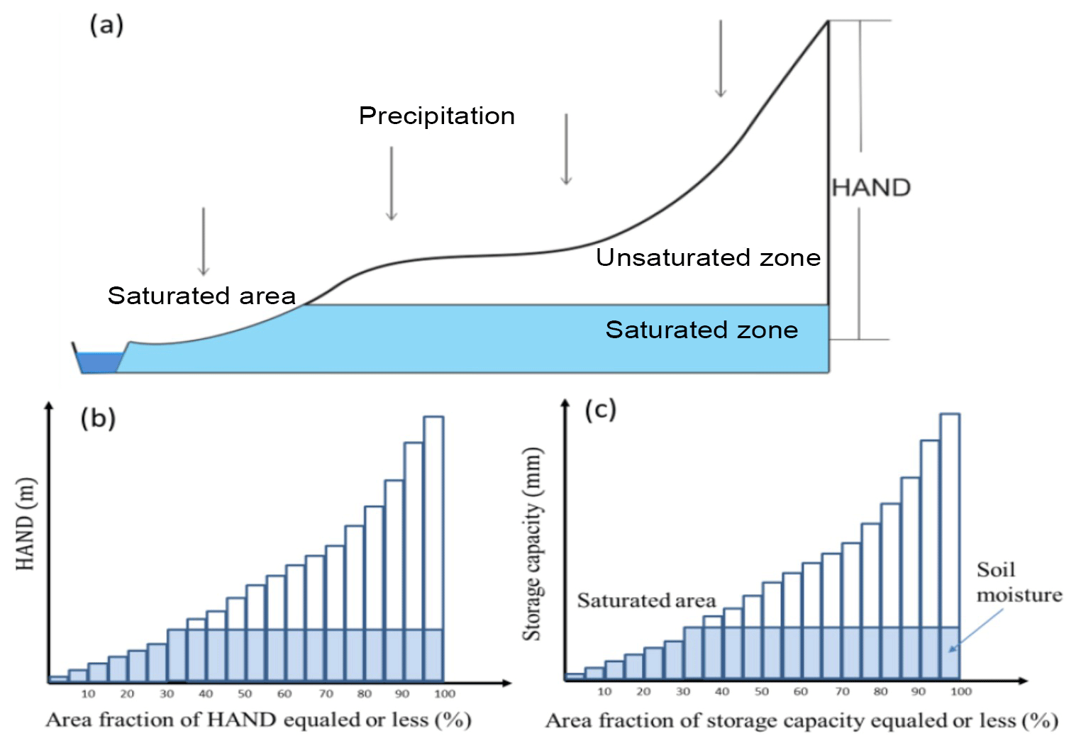
Figure 2The perceptual model of the HAND-based Storage Capacity curve (HSC) model. Panel (a) shows the representative hillslope profile in nature, and the saturated area, unsaturated zone and saturated zone; panel (b) shows the relationship between HAND bands and their corresponded area fraction; panel (c) shows the relationship between storage capacity-area fraction-soil moisture-saturated area, based on the assumption that storage capacity linearly increases with HAND values.
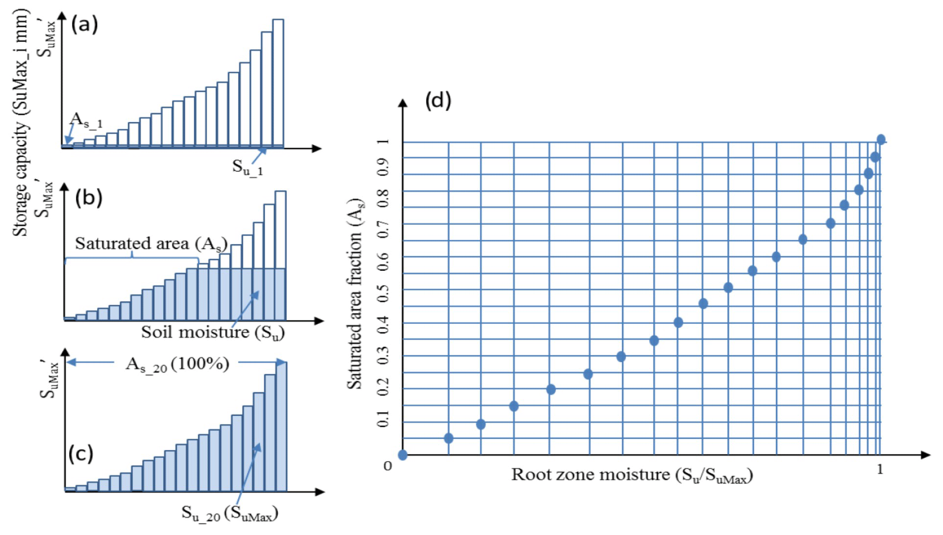
Figure 3The conceptual model of the HSC model. Panels (a), (b), and (c) illustrate the relationship between soil moisture (Su) and saturated area (As) in different soil moisture conditions. In (d), 20 different Su–As conditions are plotted, which allow us to estimate As from Su.
Figure 2 shows the perceptual HSC module, in which we simplified the complicated 3-D topography of a real catchment into a 2-D simplified hillslope. And then derive the distribution of root zone storage capacity, based on topographic analysis and the second assumption as mentioned in the preceding paragraph. Figure 3 shows the approach to derive the Su–As relation, which is detailed as follows.
- I.
Generate HAND map. The HAND map, which represents the relative vertical distance to the nearest river channel, can be generated from a DEM (Gharari et al., 2011). The stream initiation threshold area is a crucial parameter, determining the perennial river channel network (Montgomery and Dietrich, 1989; Hooshyar et al., 2016), and significantly impacting the HAND values. In this study, the start area was chosen as 40 ha for the BB catchment to maintain a close correspondence to the observed stream network. And for the MOPEX catchments, the stream initiation area threshold is set as 500 grid cells (4.05 km2), which fills in the range of stream initiation thresholds reported by others (e.g., Colombo et al., 2007; Moussa, 2008, 2009). HAND maps were then calculated from the elevation of each raster cell above the nearest grid cell flagged as a stream cell following the flow direction (Gharari et al., 2011).
- II.
Generate normalized HAND distribution curve. Firstly, sort the HAND values of grid cells in ascending order. Secondly, divide the sorted HAND values evenly into n bands (e.g., 20 bands in this study), to make sure each HAND band has a similar area. The averaged HAND value of each band is regarded as the HAND value of that band. Thirdly, normalize the HAND bands, and then plot the normalized HAND distribution curve (Fig. 2b).
- III.
Distribute SuMax to each HAND band (SuMax_i). As assumed, the normalized storage capacity of each HAND band (SuMax_i) increases with HAND value (Fig. 2c). Based on this assumption, the unsaturated root zone storage capacity (SuMax) can be distributed to each HAND band as SuMax_i (Fig. 3a). It is worth noting that SuMax needs to be calibrated in the HSC module, but free of calibration in the HSC-MCT module.
- IV.
Derive the Su−As curve. With the number of s saturated HAND bands (Fig. 3a–c), the soil moisture (Su) can be obtained by Eq. (5); and saturated area proportion (As) can be obtained by Eq. (6).
where SuMax_s is the maximum SuMax_i of all the saturated HAND bands. Subsequently, the As–Su curve can be derived, and is shown in Fig. 3d.
The SEF mechanism assumes that runoff is only generated from saturation areas; therefore, the proportion of the saturation area is equal to the runoff coefficient of that rainfall–runoff event. Based on the Su–As curve in Fig. 3d, generated runoff can be calculated from root zone moisture (Su). The HSC module also allows us to map out the fluctuation of saturated areas by the simulated catchment average soil moisture. For each time step, the module can generate the simulated root zone moisture for the entire basin (Su). Based on the Su–As relationship (Fig. 3d), we can map Su back to the saturated area proportion (As) and then visualize it in the original HAND map. Based on this conceptual model, we developed the computer program and created a procedural module. The technical roadmap can be found in Fig. 4.

Figure 4The procedures estimating runoff generation by the HSC model and its two hypotheses.
2.3 HSC-MCT module
The SuMax is an essential parameter in various hydrological models (e.g., HBV, Xinanjiang, GR4J), which determines the long-term partitioning of rainfall into infiltration and runoff. Gao et al. (2014a) found that SuMax represents the adaption of ecosystems to local climate. Ecosystems may design their SuMax based on the precipitation pattern and their water demand. The storage is neither too small to be mortal in dry seasons, nor too large to consume excessive energy and nutrients. Based on this assumption, we can estimate the SuMax without calibration, by the MCT method, from climatological and vegetation information. More specifically, the average annual plant water demand in the dry season (SR) is determined by the water balance and the vegetation phenology, i.e., precipitation, runoff, and seasonal NDVI. Subsequently, based on the annual SR, the Gumbel distribution (Gumbel, 1935), frequently used for estimating hydrological extremes, was used to standardize the frequency of drought occurrence. SR20yr, i.e., the root zone storage capacity required to overcome a drought once in 20 years, is used as the proxy for SuMax due to the assumption of a “cost” minimization strategy of plants as we mentioned above (Milly, 1994), and the fact that SR20yr has the best fit with SuMax. The SR20yr of the MOPEX catchments can be found in the map of Gao et al. (2014a).
Eventually, with the MCT approach to estimate SuMax and the HSC curve to represent the root zone storage capacity spatial distribution, the HSC-MCT runoff generation module is created, without free parameters. It is worth noting that both the HSC-MCT and HSC modules are based on the HAND-derived Su–As relation, and their distinction lays in the methods to obtain SuMax. So far, the HBV power function module has two free parameters (SuMax, β), while the TOPMODEL and the HSC both have one free parameter (SuMax). Ultimately the HSC-MCT has no free parameter.
2.4 Interception, evaporation and routing modules
Except for the runoff generation module in the root zone reservoir (SUR), we need to consider other processes, including interception (SIR) before the SUR module, evaporation from the SUR and the response routine (SFR and SSR) after runoff generation from SUR (Fig. 5). Precipitation is firstly intercepted by vegetation canopies. In this study, the interception was estimated by a threshold parameter (SiMax), set to 2 mm (Gao et al., 2014a), below which all precipitation will be intercepted and evaporated (Eq. 9) (de Groen and Savenije, 2006). For the SUR reservoir, we can either use the HBV beta-function (Eq. 12), the runoff generation module of TOPMODEL (Eqs. 2–4) or the HSC module (Sect. 2.3) to partition precipitation into generated runoff (Ru) and infiltration. The actual evaporation (Ea) from the soil equals the potential evaporation (Ep), if Su∕SuMax is above a threshold (Ce), where Su is the soil moisture and SuMax is the catchment-averaged storage capacity. And Ea linearly reduces with Su∕SuMax, while Su∕SuMax is below Ce (Eq. 13). The Ep can be calculated by the Hargreaves equation (Hargreaves and Samani, 1985), with maximum and minimum daily temperature as input. The generated runoff (Ru) is further split into two fluxes, including the flux to the fast response reservoir (Rf) and the flux to the slow response reservoir (Rs), by a splitter (D) (Eq. 14). The delayed time from rainfall peak to the flood peak is estimated by a convolution delay function, with a delay time of TlagF (Eqs. 15, 16). Subsequently, the fluxes into two different response reservoirs (SFR and SSR) were released by two linear equations between discharge and storage (Eqs. 18, 21), representing the fast response flow and the slow response flow mainly from groundwater reservoir. The two discharges (Qf and Qs) generated the simulated streamflow (Qm). The model parameters are shown in Table 1, while the equations are given in Table 2. More detailed description of the model structure can be referred to Gao et al. (2014b, 2016). It is worth underlining that the only difference among the benchmark HBV type, TOPMODEL type, HSC, and HSC-MCT models is their runoff generation modules. Eventually, there are 7 free parameters in HBV model, 6 in TOPMODEL and HSC model, and 5 in the HSC-MCT model.
Table 1The parameters of the models, and their prior ranges for calibration.
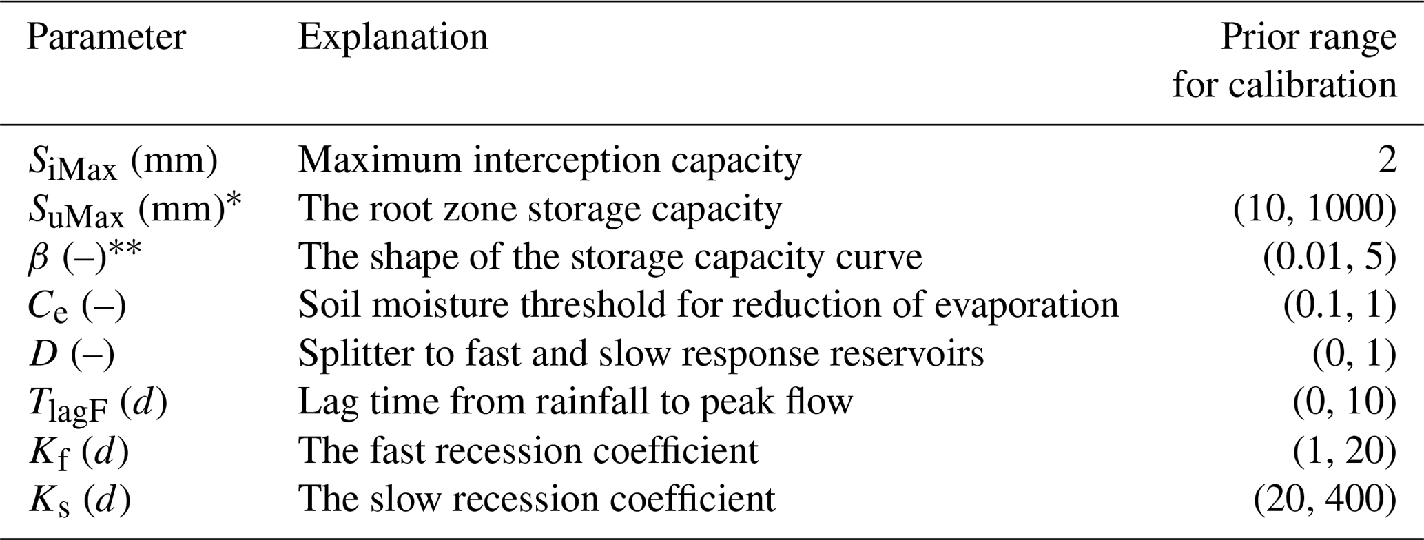
* SuMax is a parameter in HBV, TOPMODEL, and the HSC model, but the HSC-MCT model does not have SuMax as a free parameter; β is a parameter in the HBV model, but not in the TOPMODEL, HSC, and HSC-MCT models.
Table 2The water balance and constitutive equations used in models. (Eq. (12)* is used in the HBV model, but is not used in the TOPMODEL, HSC, and HSC-MCT models).
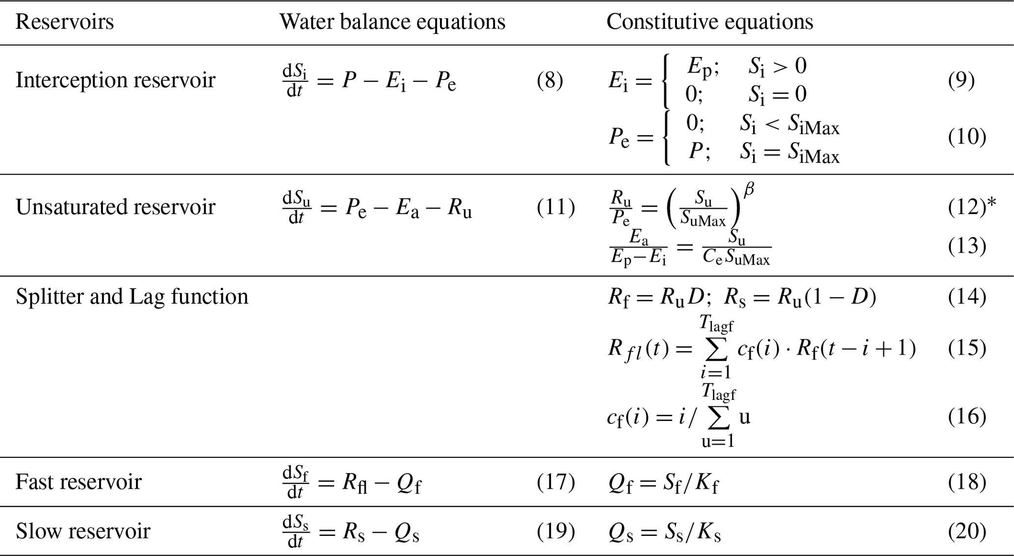
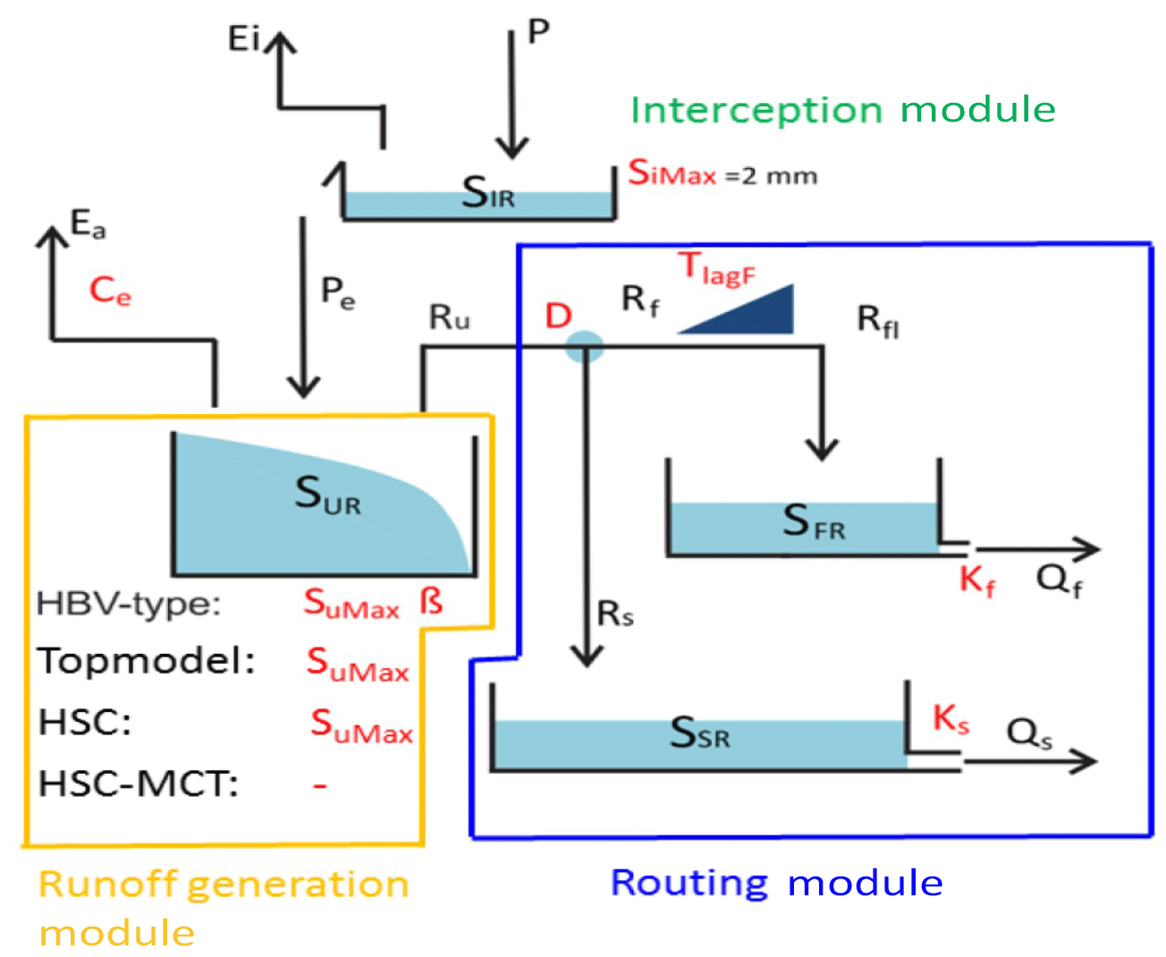
Figure 5Model structure and free parameters, involving four runoff generation models (HBV-type, TOPMODEL, HSC, and HSC-MCT). HBV-type has SuMax and beta two free parameters; TOPMODEL and HSC models have SuMax as one free parameter; and the HSC-MCT model does not have a free parameter. In order to simplify calibration process and make fair comparison, the interception storage capacity (SiMax) was fixed as 2 mm.
2.5 Model evaluation, calibration, validation, and model comparison
Two objective functions were used to evaluate model performance, since multi-objective evaluation is a more robust approach to quantifying model performance with different criteria than a single one. The Kling–Gupta efficiency (Gupta et al., 2009) (IKGE) was used as the criterion to evaluate model performance and as an objective function for calibration. The equation is written as
where r is the linear correlation coefficient between simulation and observation; α () is a measure of relative variability in the simulated and observed values, where σm is the standard deviation of simulated streamflow, and σo is the standard deviation of observed streamflow; and ε is the ratio between the average value of simulated and observed data. And the IKGL (IKGE of the logarithmic flows) (Fenicia et al., 2007; Gao et al., 2014b) is used to evaluate the model performance in baseflow simulation.
A multi-objective parameter optimization algorithm (MOSCEM-UA) (Vrugt et al., 2003) was applied for the calibration. The parameter sets on the Pareto-frontier of the multi-objective optimization were assumed to be the behavioral parameter sets and can equally represent model performance. The averaged hydrograph obtained by all the behavioral parameter sets were regarded as the simulated result of that catchment for further studies. The number of complexes in MOSCEM-UA were set as the number of parameters (seven for HBV, six for TOPMODEL and the HSC model, and five for the HSC-MCT model), and the number of initial samples was set to 210 and a total number of 50 000 model iterations for all the catchment runs. For each catchment, the first half period of data was used for calibration, and the other half was used to do validation.
In module comparison, we defined three categories: if the difference of IKGE of model A and model B in validation is less than 0.1, model A and B are regarded as “equally well”. If the IKGE of model A is larger than model B in validation by 0.1 or more, model A is regarded as outperforming model B. If the IKGE of model A is less than model B in validation by −0.1 or less, model B is regarded as outperforming model A.
3.1 The Bruntland Burn catchment
The 3.2 km2 Bruntland Burn catchment (Fig. 6), located in north-eastern Scotland, was used as a benchmark study to test the model's performance based on a rich data base of hydrological measurements. The Bruntland Burn is a typical upland catchment in northwestern Europe (e.g., Birkel et al., 2010), namely a combination of steep and rolling hillslopes and over-widened valley bottoms due to the glacial legacy of this region. The valley bottom areas are covered by deep (in parts >30 m) glacial drift deposits (e.g., till) containing a large amount of stored water superimposed on a relatively impermeable granitic solid geology (Soulsby et al., 2016). Peat soils developed (>1 m deep) in these valley bottom areas, which remain saturated throughout most of the year with a dominant near-surface runoff generation mechanism delivering runoff quickly via micro-topographical flow pathways connected to the stream network (Soulsby et al., 2015). Brown rankers, peaty rankers and peat soils are responsible for a flashy hydrological regime driven by saturation excess overland flow, while humus iron podzols on the hillslopes do not favor near-surface saturation but rather facilitate groundwater recharge through vertical water movement (Tetzlaff et al., 2014). Land use is dominated by heather moorland, with smaller areas of rough grazing and forestry on the lower hillslopes. Its annual precipitation is 1059 mm, with the summer months (May–August) generally being the driest (Ali et al., 2014). Snow makes up less than 10 % of annual precipitation and melts rapidly below 500 m. The evapotranspiration is around 400 mm per year and annual discharge around 659 mm. The daily precipitation, potential evaporation, and discharge data range from 1 January 2008 to 30 September 2014. The calibration period is from 1 January 2008 to 31 December 2010, and the data from 1 January 2011 to 30 September 2014 is used as validation.
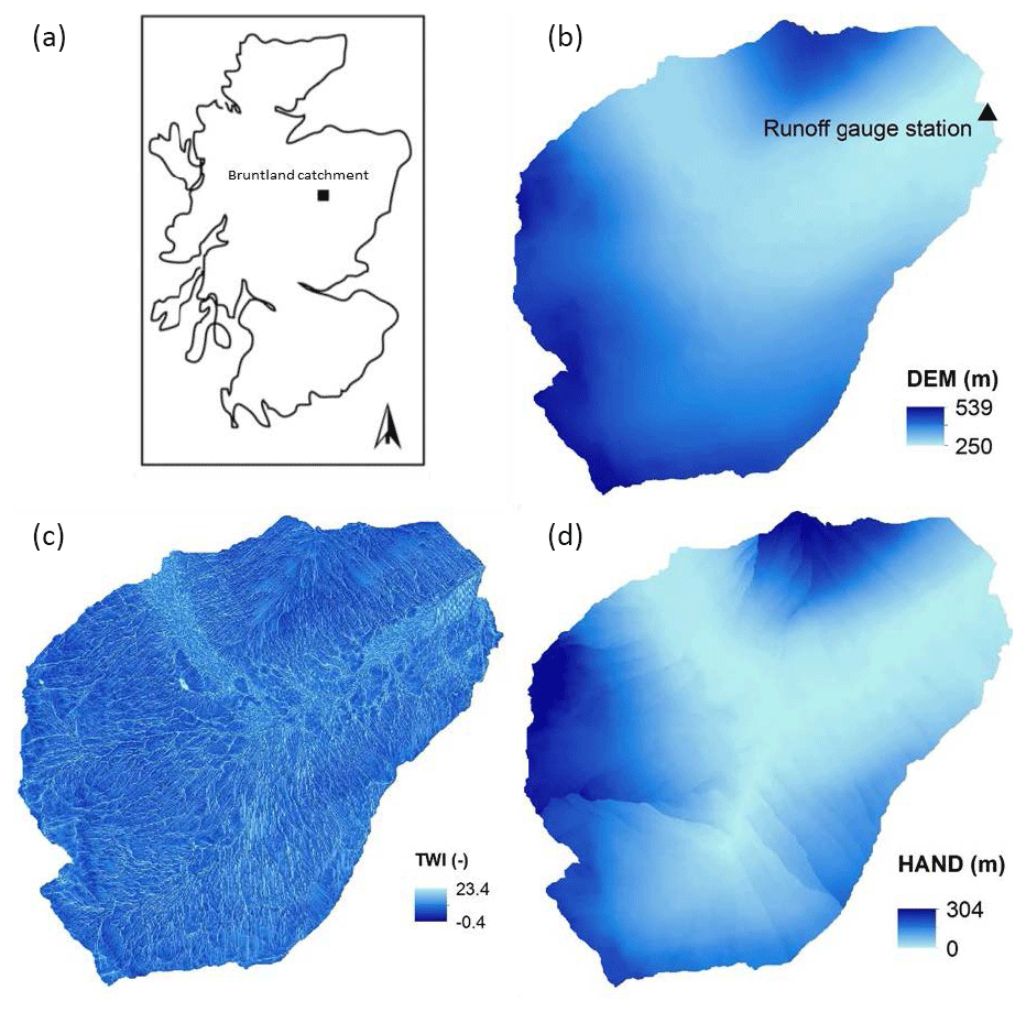
Figure 6(a) Study site location of the Bruntland Burn catchment within Scotland; (b) digital elevation model (DEM) of the Bruntland Burn catchment; (c) the topographic wetness index map of the Bruntland Burn catchment; (d) the HAND map of the Bruntland Burn catchment.
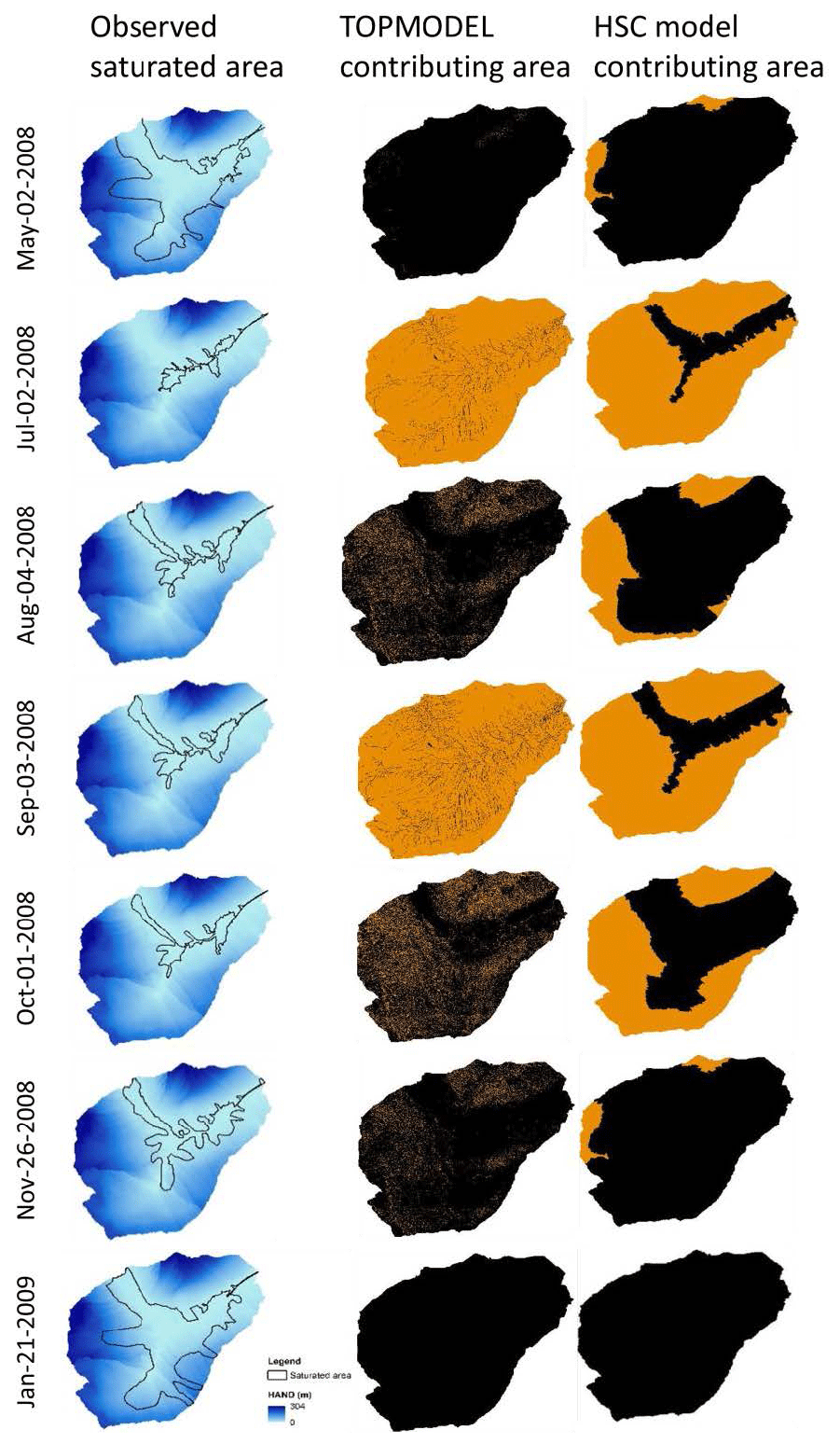
Figure 7The measured saturated areas and the simulated contributing areas (black) by TOPMODEL and HSC models.
The LiDAR-derived DEM map with 2 m resolution shows elevation ranging from 250 to 539 m (Fig. 6). There are seven saturation area maps (Fig. 7) (2 May, 2 July, 4 August, 3 September, 1 October, 26 November 2008, and 21 January 2009), measured directly by the “squishy boot” method and field mapping by the global positioning system (GPS), to delineate the boundary of saturation areas connected to the stream network (Birkel et al., 2010; Ali et al., 2014). These saturation area maps revealed a dynamic behavior of expanding and contracting areas connected to the stream network that were used as a benchmark test for the HSC module.
3.2 MOPEX catchments
The MOPEX dataset was collected for a hydrological model parameter estimation experiment (Duan et al., 2006; Schaake et al., 2006), containing 438 catchments in the CONUS (Contiguous United States). The longest time series range from 1948 to 2003. 323 catchments were used in this study (see the name list in SI), with areas between 67 and 10 329 km2, and excluding the catchments with data records <30 years, impacted by snowmelt or with extreme arid climate (aridity index Ep∕P>2). In order to analyze the impacts of catchment characteristics on model performance, excluding hydrometeorology data, we also collected the datasets of topography, depth to rock, soil texture, land use, and stream density (Table 3). These characteristics help us to understand in which catchments the HSC performs better or worse than the benchmark models.
Table 3Data source of the MOPEX catchments. All links in this table were last accessed on 6 February 2017.
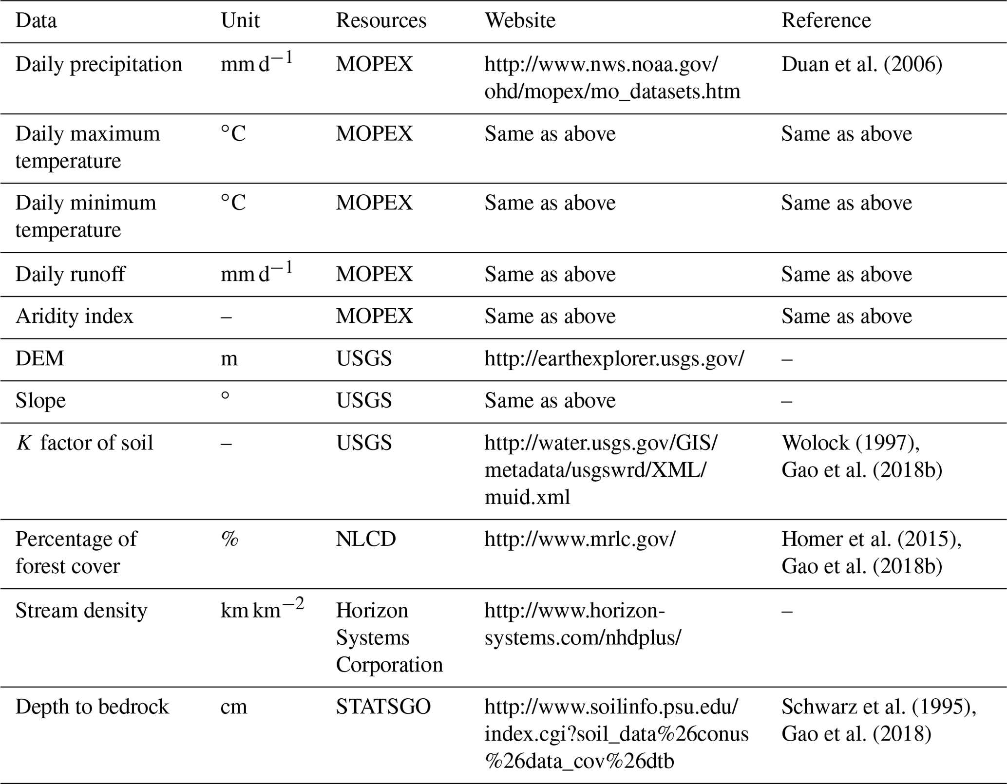
Hydrometeorology
The dataset contains the daily precipitation, daily maximum and minimum air temperature, and daily streamflow. The daily streamflow was used to calibrate the free parameters and validate the models.
Topography
The DEM of the CONUS in 90 m resolution was download from the Earth Explorer of United States Geological Survey (USGS, http://earthexplorer.usgs.gov/, last access: 25 April 2017). The HAND and TWI map can be generated from the DEM. The averaged elevation and HAND are used as two catchment characteristics.
Soil texture
In this study, soil texture is synthetically represented by the K factor, since the K factor is a lumped soil erodibility factor which represents the soil profile reaction to soil detachment (Renard et al., 2011). Generally, the soils (high in clay and sand) have low K values, and soils with high silt content have larger K values. The averaged K factor for each catchment was calculated from soil survey information available from USGS (Wolock, 1997).
Land use
Land use data was obtained from National Land Cover Database (NLCD, Wickham et al., 2014). Forest plays an essential role in hydrological processes (Gao et al., 2018a), especially for the runoff generation (Brooks et al., 2010). Forest area proportion was utilized as an integrated indictor to represent the impact of vegetation cover on hydrological processes.
Stream density
Stream density (km km−2) is the total length of all the streams and rivers in a drainage basin divided by the total area of the drainage basin. Stream density data was obtained from Horizon Systems Corporation (http://www.horizon-systems.com/nhdplus/, last access: 25 April 2017).
Geology
Bedrock is a relative impermeable layer, as the lower boundary of subsurface stormflow in the catchments where soil depth is shallow (Tromp-van Meerveld and McDonnell, 2006). The depth to bedrock, as an integrated geologic indicator, was accessed from STATSGO (State Soil Geographic, http://www.soilinfo.psu.edu/index.cgi?soil_data\%26conus\%26data_cov\%26dtb, last access: 25 April 2017) (Schwarz and Alexander, 1995). The averaged depth to bedrock for each catchment was calculated for further analysis.
4.1 Topography analysis
The generated HAND map, derived also from the DEM, is shown in Fig. 6, with HAND values ranging from 0 to 234 m. Based on the HAND map, we can derive the Su–As curve (Fig. 8) by analyzing the HAND map with the method in Sect. 2.3. The TWI map of the BB (Fig. 6) was generated from its DEM. Overall, the TWI map, ranging from −0.4 to 23.4, mainly differentiates the valley bottom areas with the highest TWI values from the steeper slopes. This is probably caused by the fine resolution of the DEM map in 2 m, as previous research found that the sensitivity of TWI to DEM resolution (Sørensen and Seibert, 2007). From the TWI map, the frequency distribution function and the accumulative frequency distribution function can be derived (Fig. 8), with one unit of TWI as the interval.
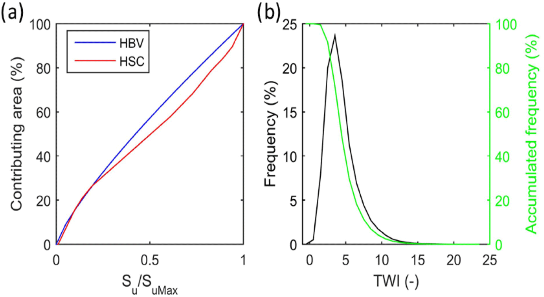
Figure 8The curves of the beta function of the HBV model, and the Su–As curve generated by the HSC model (a). The frequency and accumulated frequency of the TWI in the Bruntland Burn catchment (b).
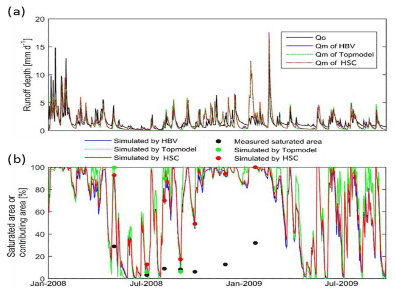
Figure 9(a) The observed hydrograph (Qo, black line) of the Bruntland Burn catchment in 2008, and the simulated hydrographs (Qm) by the HBV model (blue line), TOPMODEL (green dash line), and HSC model (red dash line); (b) the comparison of the observed saturated area of 7 days (black dots) and simulated relative soil moistures, i.e., HBV (blue line), TOPMODEL (green line and dots), and HSC (red line and dots).
4.2 Model performance
It is found that all three models (HBV, TOPMODEL, and HSC) can perform well in reproducing the observed hydrograph (Fig. 9). The IKGE of the three models are all around 0.66 in calibration, which is largely in line with other studies from the BB (Birkel et al., 2010, 2014). And the IKGL are 0.76, 0.72, and 0.74 for HSC, HBV, and TOPMODEL, respectively, in calibration, while in validation, the IKGE of the three models are also around 0.66, while IKGL are 0.75, 0.70, and 0.65 for the three models. Since the measured rainfall–runoff time series only lasts from 2008 to 2014, which is too short to estimate the SR20yr (proxy for SuMax) by the MCT approach (which needs long-term hydro-meteorological observation data), the HSC-MCT model was not applied to this catchment.
Figure 8 shows the calibrated power curve by HBV (averaged beta =0.98) with the Su–As curve obtained from the HSC module. We found the two curves are largely comparable, especially while the relative soil moisture is low. This result demonstrates that for the BB catchment with glacial drift deposits and combined terrain of steep and rolling hillslopes and over-widened valley bottoms, the HBV power curve can essentially be derived from the Su–As curve of the HSC module merely by topographic information without calibration.
The normalized relative soil moisture of the three model simulations are presented in Fig. 9. Their temporal fluctuation patterns are comparable. Nevertheless, the simulated soil moisture by TOPMODEL has larger variation, compared with HBV and HSC (Fig. 9).
4.3 Contributing area simulation
The observed saturation area and the simulated contributing area from both TOPMODEL and the HSC are shown in Figs. 7, 9, and 10. We found that, although both modules overestimated the saturated areas, they can capture the temporal variation. For example, the smallest saturated area, both observed and simulated, occurred on 2 July 2008, and the largest saturated areas both occurred on 21 January 2009. Comparing the estimated contributing area of TOPMODEL with the HSC module, we found that the results of the HSC correlate better (R2=0.60, ) with the observed saturated areas than TOPMODEL (R2=0.50, ) (Fig. 10). For spatial patterns, the HSC contributing area is located close to the river network and reflects the spatial pattern of observed saturated area, while TOPMODEL results are more scattered, probably due to the sensitivity of TWI to DEM resolution (Fig. 7). The HSC is more discriminating in terms of less frequently giving an unrealistic 100 % saturation and retaining unsaturated upper hillslopes.
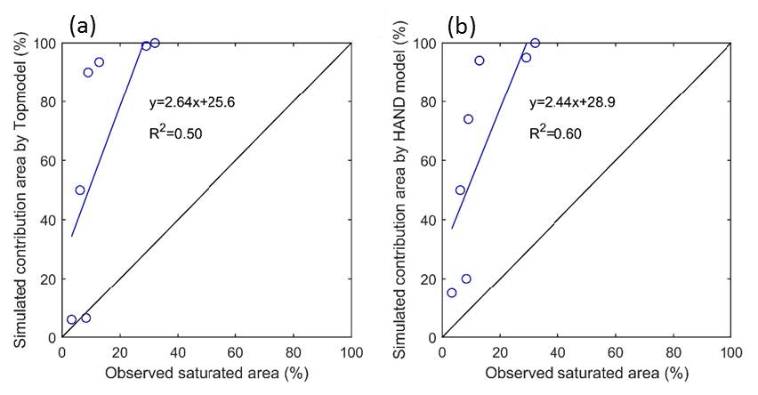
Figure 10The comparison of the observed saturated area and simulated contributing areas by the TOPMODEL and HSC models.
5.1 Topography analysis of the contiguous US and 323 MOPEX catchments
To delineate the TWI map for the CONUS, the depressions of the DEM were firstly filled with a threshold height of 100 m (recommended by Esri). The TWI map of the CONUS is produced (Fig. S1 in the Supplement). Based on the TWI map of the CONUS, we clipped the TWI maps for the 323 MOPEX catchments with their catchment boundaries. And then the TWI frequency distribution and the accumulated frequency distribution of the 323 MOPEX catchments (Fig. S2), with one unit of TWI as an interval, were derived based on the 323 TWI maps.
In Fig. 11, it is shown that the regions with large HAND values are located in Rocky Mountains and Appalachian Mountains, while the Great Plains has smaller HAND values. The Great Basin, especially in the Salt Lake Desert, has small HAND values, illustrating its low elevation above the nearest drainage, despite a high elevation above sea level. From the CONUS HAND map, we clipped the HAND maps for the 323 MOPEX catchments with their catchment boundaries. We then plot their HAND-area curves, following the procedures of I and II in Sect. 2.2. Figure 12a shows the normalized HAND profiles of the 323 catchments.
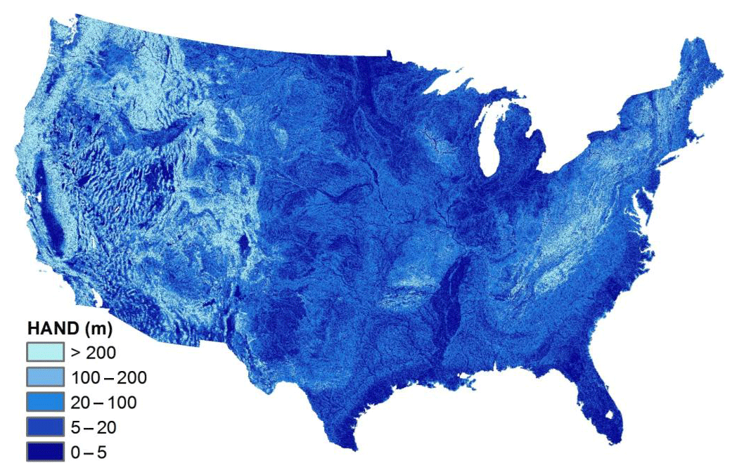
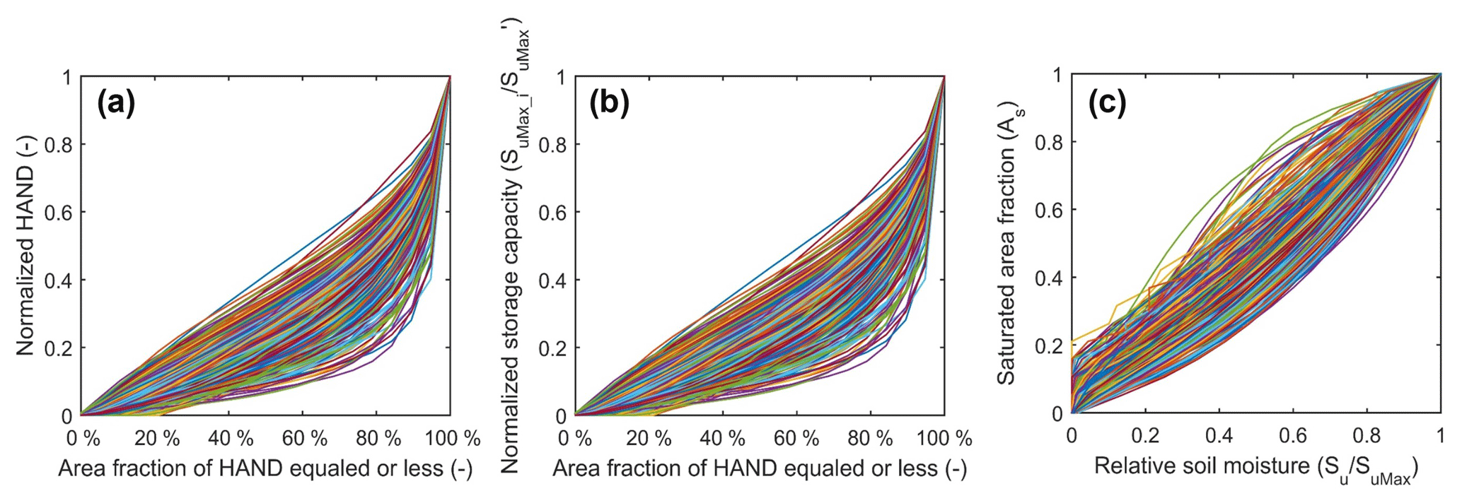
Figure 12(a) The profiles of the normalized HAND of the 323 MOPEX catchments; (b) the relations between area fraction and the normalized storage capacity profile of the 323 MOPEX catchments; (c) the Su–As curves of the HSC model which can be applied to estimate runoff generation from relative soil moisture for the 323 MOPEX catchments.
Based on the HAND profiles and the Step III in Sect. 2.2, we derived the normalized storage capacity distribution for all catchments (Fig. 12b). Subsequently, the root zone moisture and saturated area relationship (As–Su) can be plotted by the method in Step IV of Sect. 2.2. Lastly, reversing the curve of As–Su to the Su–As relation (Fig. 12c), the latter can be implemented to simulate runoff generation by soil moisture. Figure 12c interestingly shows that in some catchments, there is almost no threshold behavior between rainfall and runoff generation, where the catchments are covered by large areas with low HAND values and limited storage capacity. Therefore, when rainfall occurs, wetlands response quickly and generate runoff without a precipitation–discharge threshold relationship characteristic of areas with higher moisture deficits. This is similar to the idea of FLEX-Topo where the storage capacity is distinguished between wetlands and hillslopes, and on wetlands, with low storage capacity, where runoff response to rainfall is almost instantaneous.
5.2 Model performance
Overall, the performance of the two benchmark models, i.e., HBV and TOPMODEL, for the MOPEX data (Fig. 13) is comparable with the previous model comparison experiments, conducted with four rainfall–runoff models and four land surface parameterization schemes (Duan et al., 2006; Kollat et al., 2012; Ye et al., 2014). The median value of IKGE of the HBV type model is 0.61 for calibration in the 323 catchments (Fig. 13), and averaged IKGE in calibration is 0.62. In validation, the median and averaged values of IKGE are kept the same as calibration. The comparable performance of models in calibration and validation demonstrates the robustness of benchmark models and the parameter optimization algorithm (i.e., MOSCEM-UA). The TOPMODEL improves the median value of IKGE from 0.61 (HBV) to 0.67 in calibration, and from 0.61 (HBV) to 0.67 in validation. But the averaged values of IKGE for TOPMODEL are slightly decreased from 0.62 (HBV) to 0.61 in both calibration and validation. The HSC module, by involving the HAND topographic information without calibrating the β parameter, improves the median value of IKGE to 0.68 for calibration and 0.67 for validation. The averaged values of IKGE in both calibration and validation are also increased to 0.65, comparing with HBV (0.62) and TOPMODEL (0.61). Furthermore, Fig. 13 demonstrates that, comparing with the benchmark HBV and TOPMODEL, not only the median and averaged values were improved by the HSC module, but also the 25th and 75th percentiles and the lower whisker end, all have been improved. The performance gains on baseflow (IKGL) have been investigated and shown in the Fig. S3. These results indicate the HSC module improved model performance to reproduce hydrograph for both peak flow (IKGE) and baseflow (IKGL).

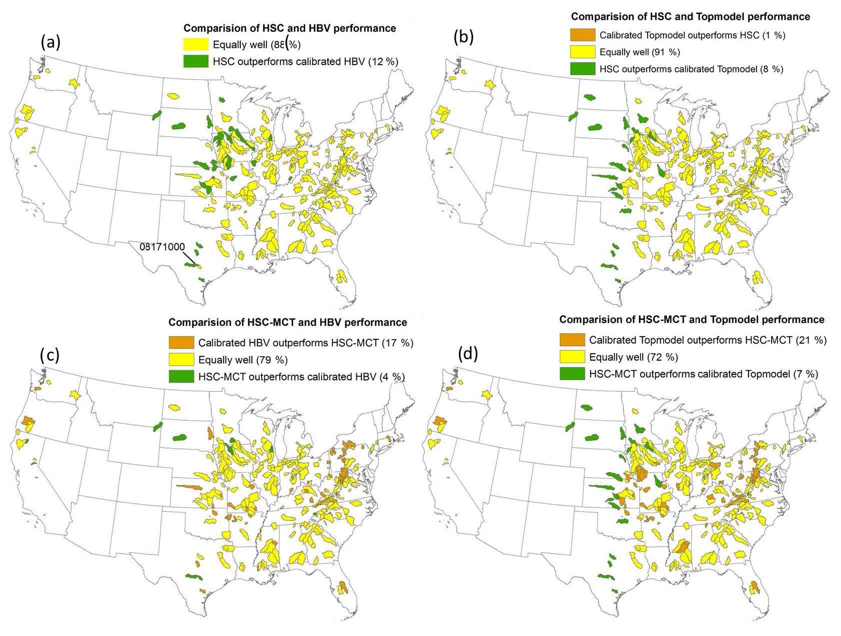
Figure 14Performance comparison of the HSC and HSC-MCT models compared to two benchmark models, HBV and TOPMODEL, for the 323 MOPEX catchments.
Additionally, for the HSC-MCT model, the median IKGE value is improved from 0.61 (HBV) to 0.65 in calibration, and from 0.61 (HBV) to 0.64 in validation, but is not as well performed as TOPMODEL (0.67 for calibration and validation). For the averaged IKGE values, they were slightly reduced from 0.62 (HBV) and 0.61 (TOPMODEL) to 0.59 for calibration and validation. Although the HSC-MCT did not perform as well as the HSC module, considering there is no free parameter to calibrate, the median IKGE value of 0.64 (HBV is 0.61) and averaged IKGE of 0.59 (TOPMODEL is 0.61) are quite acceptable. In addition, the 25th and 75th percentiles and the lower whisker end of the HSC-MCT model are all improved compared to the HBV model. Moreover, the largely comparable results between the HSC and the HSC-MCT modules demonstrate the feasibility of the MCT method to obtain the SuMax parameter and the potential for HSC-MCT to be implemented in prediction of ungauged basins.
Figure 14 shows the spatial comparisons of the HSC and HSC-MCT models with the two benchmark models. We found that the HSC performs “equally well” as HBV (the difference of IKGE in validation ranges −0.1–0.1) in 88 % catchments, and in the remaining 12 % of the catchments the HSC outperforms HBV (the improvement of IKGE in validation is larger than 0.1). In not a single catchment did the calibrated HBV outperform the HSC. Comparing the HSC model with TOPMODEL, we found in 91 % of the catchments that the two models have approximately equal performance. In 8 % of the catchments, the HSC model outperformed TOPMODEL. Only in 1 % of the catchments (two in the Appalachian Mountains and one in the Rocky Mountains in California), TOPMODEL performed better.
Table 4Impacts of MOPEX catchment characteristics on model performance (HSC, HBV, and TOPMODEL).
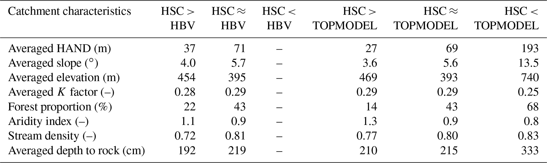
In order to further explore the impact of catchment characteristics on model performance, we used topography (averaged HAND, averaged slope, and averaged elevation), soil (K factor), land cover (forest area proportion), climate (aridity index), stream density, and geology (depth to rock) information to test the impact of catchment features on model performance. Table 4 clearly shows that compared with HBV, the 39 catchments with better performance have lower HAND values (37 m), more gentle slopes (4.0∘), and smaller forest area (22 %); while the elevation, K factor, aridity index, stream density and depth to rock are almost similar. Also, in the catchments where HSC outperformed TOPMODEL, the catchments have smaller HAND (27 m), more gentle slopes (3.6∘), moderate elevation (469 m), less forest proportion (14 %), and more arid climate (aridity index is 1.3). TOPMODEL performs better in only three catchments with larger HAND (193 m), steeper slopes (13.5∘), higher elevation (740 m), more humid climate (aridity index is 0.8), and larger depth to rock (333 cm). In summary, the HSC showed better performance in catchments with gentle topography and more arid climate.
Without calibration of SuMax, as expected, the performance of the HSC-MCT module slightly deteriorates (Fig. 13). In comparison with HBV, the outperformed percentage reduced from 12 % (HSC) to 4 % (HSC-MCT), the approximately equally well-simulated catchments dropped from 88 % to 79 %, and the inferior performance increased from 0 % to 17 %. Also, in comparison with TOPMODEL, the better performance dropped from 8 % (HSC) to 7 % (HSC-MCT), the approximately equal catchments reduced from 91 % to 72 %, and the inferior performance increased from 1 % to 21 %. The inferiority of the HSC-MCT model is probably caused by the uncertainty of the MCT method for different ecosystems which have different survival strategies and use different return periods to bridge critical drought periods. By using ecosystem dependent return periods, this problem could be reduced (Wang-Erlandsson et al., 2016).
To further explore the reason for the better performance of the HSC approach, we selected the 08171000 catchment in Texas (Fig. 14), in which both the HSC module and the HSC-MCT module outperformed the two benchmark modules to reproduce the observed hydrograph (Fig. S4). The HBV model dramatically underestimated the peak flows, with IKGE as 0.54, while TOPMODEL significantly overestimated the peak flows, with IKGE as 0.30. The HSC-MCT model improved the IKGE to 0.71, and the HSC model further enhanced IKGE to 0.74.
Since the modules of interception, evaporation and routing are identical for the four models, the runoff generation modules are the key to understand the difference in model performance. Figure S5 shows the HBV β curve and the Su–As curve of the HSC model, as well as the TWI frequency distribution. We found that with a given Su∕SuMax, the HBV β function generates less contributing area than the HSC model, which explains the underestimation of the HBV model. In contrast, TOPMODEL has a sharp and steep accumulated TWI frequency curve. In particular, the region with TWI =8 accounts for 40 % of the catchment area, and over 95 % of the catchment areas are within the TWI ranging from 6 to 12. This indicates that even with low soil moisture content (Su∕SuMax), the contributing area by TOPMODEL is relatively large, leading to the sharply increased peak flows for all rainfall events.
6.1 Rainfall–runoff processes and topography
We applied a novel approach to derive the relationship between soil moisture storage and the saturated area from HAND. The areas with relatively low HAND values are saturated earlier than areas with higher HAND values, due to the larger storage capacity in higher HAND locations. The outperformance of the HSC over the benchmark HBV and TOPMODEL in gentle sloping catchments indicates that the HSC module likely has a higher realism than the calibrated HBV beta-function and the TWI of TOPMODEL in these regions. Very interestingly, Fan et al. (2017) presented an ecological observation in the global scale, and revealed the systematic variation of rooting depth along HAND (Fig. 1, in Fan et al., 2017). Since rooting depth can be translated to root zone storage capacity through combination with soil plant-available water (Wang-Erlandsson et al., 2016). This large sample dataset, from an ecological perspective, provides strong support for the assumption of the HSC model on gentle slopes, i.e., the increase in root zone storage capacity with HAND. More interestingly, on excessively drained uplands, rooting depth does not follow the same pattern, with shallow depth and limited to rain infiltration (Fig. 1, in Fan et al., 2017). This could explain the inferior performance of HSC model to TOPMODEL in three MOPEX catchments with excessively drained uplands (larger HAND, steeper slope, higher elevation, and deeper depth to rock), where Hortonian overland flow is likely the dominant mechanism, and the HSC assumption likely does not work well. This indicates that comparing with TWI, the HAND is closer to catchment realism distinguishing hydrological similarity in gentle topography catchments. The HSC module assumes SEF as the dominant mechanism. But since in a real catchment different runoff generating processes may act simultaneously in different environments (McDonnell, 2013; Hrachowitz and Clark, 2017). Such SEF dominated catchments, or parts thereof, are typically characterized by a subdued relief and thus gently sloping. In steeper catchments, where the groundwater table is deeper and thus more additional water can be stored in the soil, another conceptual parameterization would be appropriate.
The FLEX-Topo model (Savenije, 2010) also uses HAND as a topographic index to distinguish between landscape-related runoff processes and has both similarity and differences with the HSC model. The results of the HSC model illustrate that the riparian areas are more prone to be saturated, which is consistent with the concept of the FLEX-Topo model. Another important similarity of the two models is their parallel model structure. In both models it is assumed that the upslope area has larger storage capacity, therefore the upper land generates runoff less and later than the lower land. In other words, in most cases, the local storage is saturated due to the local rainfall, instead of flow from upslope. The most obvious difference between the HSC and the FLEX-Topo is the approach towards discretization of a catchment. The FLEX-Topo model classifies a catchment into various landscapes, e.g., wetlands, hillslopes, and plateau. This discretization method requires threshold values to classify landscapes, i.e., threshold values of HAND and slope, which leads to fixed and time-independent proportions of landscapes. The HSC model does not require landscape classification, which reduced the subjectivity in discretization and restricted the model complexity, as well as simultaneously allowing the fluctuation of contributing areas (termed as wetlands in FLEX-Topo).
6.2 Catchment heterogeneity and simple models
Catchments exhibit a wide array of heterogeneity and complexity with spatial and temporal variations of landscape characteristics and climate inputs. For example, the Darcy–Richards equation approach is often consistent with point-scale measurements of matrix flow, but not for preferential flow caused by roots, soil fauna, and even cracks and fissures (Beven and Germann, 1982; Zehe and Fluehler, 2001; Weiler and McDonnell, 2007). As a result, field experimentalists continue to characterize and catalog a variety of runoff processes, and hydrological and land surface modelers are developing more and more complicated models to involve the increasingly detailed processes (McDonnell et al., 2007). However, there is still no compelling evidence to support the outperformance of sophisticated “physically based” models in terms of higher equifinality and uncertainty than the simple lumped or semi-distributed conceptual models in rainfall–runoff simulation (Beven, 1989; Orth et al., 2015).
But evidence is mounting that a catchment is not a random assemblage of different heterogeneous parts (Sivapalan, 2009; Troch et al., 2013; Zehe et al., 2013), and conceptualizing heterogeneities does not require complex laws (Chase, 1992; Passalacqua et al., 2015). Parsimonious models (e.g., Perrin et al., 2003), with empirical curve shapes, likely result in good model performance. Parameter identifiability in calibration is one of the reasons. However, the physical rationale of these parsimonious models is still largely unknown, lacking a physical explanation to interpret these empirical curves described by mathematical functions (e.g., Eq. 3 in Perrin et al., 2003).
The benefits of the new HSC module are 2-fold. From a technical point of view, the HSC allows us to make prediction in ungauged basins without calibrating the beta parameter in many conceptual hydrological models. Furthermore, the HSC module, from a scientific point of view, provides us with a new perspective on the linkage between the spatial distribution patterns of root zone storage capacity (long-term ecosystem evolution) with associated runoff generation (event-scale rainfall–runoff generation).
Asking questions of “why” rather than “what” likely leads to more useful insights and a new way forward (McDonnell et al., 2007). The HSC module provides us with a rationale from an ecological perspective to understand the linkage and mechanism between large-sample hillslope ecological observations and the curve of root zone storage capacity distribution (Figs. 1, 2, and 3). Catchment is a geomorphological and even an ecological system whose parts are related to each other probably due to catchment self-organization and evolution (Sivapalan and Blöschl, 2015; Savenije and Hrachowitz, 2017). This encourages the hope that simplified concepts may be found adequate to describe and model the operation of the basin runoff generation process. It is clear that topography, with fractal characteristic (Rodriguez-Iturbe and Rinaldo, 1997), is often the dominant driver of runoff, as well as being a good integrated indicator for vegetation cover (Gao et al., 2014b), rooting depth (Fan et al., 2017), root zone evaporation and transpiration deficits (Maxwell and Condon, 2016), soil properties (Seibert et al., 2007), and even geology (Rempe and Dietrich, 2014; Gomes, 2016). Therefore, we argue that increasingly detailed topographic information is an excellent integrated indicator allowing modelers to continue systematically represent heterogeneities and simultaneously reduce model complexity. The model structure and parameterization of both HSC and TOPMODEL are simple, but not oversimplified, as they capture likely the most dominant factor controlling runoff generation, i.e., the spatial heterogeneity of storage capacity. Hence, this study also sheds light on the possibility of moving beyond heterogeneity and process complexity (McDonnell et al., 2007), to simplify them into a succinct and a priori curve by taking advantage of catchment self-organization probably caused by co-evolution (Wang and Tang, 2014) or the principle of maximum entropy production (Kleidon and Lorenz, 2004).
6.3 Implications and limitation
The calibration-free HSC-MCT runoff generation module enhances our ability to predict runoff in ungauged basins. PUB is probably not a major issue in the developed world, with abundant comprehensive measurements in many places, but for the developing world it requires prediction with sparse data and fragmentary knowledge. Topographic information with high spatial resolution is freely available globally, allowing us to implement the HSC model in global-scale studies. In addition, thanks to the recent development, testing, and validation of remote sensing precipitation and evaporation products at large spatial scales (e.g., Anderson et al., 2011; Hu and Jia, 2015; Duan et al., 2019), the SuMax estimation has become possible without in situ hydro-meteorological measurements (Wang-Erlandsson et al., 2016). These widely accessible datasets make the global-scale implementation of the HSC-MCT module promising.
Although the new modules perform well in the BB and the MOPEX catchments, we do not intend to propose that “a model fits all”. The assumption of HSC, to some extent, is supported by large-sample ecological field observation (Fan et al., 2017), but it never means that the As–Su curve of HSC can perfectly fit the other existing curves (e.g., HBV and TOPMODEL). Unifying all model approaches into one framework is the objective of several pioneer works (e.g., Clark, et al., 2008; Fenicia et al., 2011), but is beyond the scope of this study. Moreover, while estimating the runoff coefficient by the As–Su relation, rainfall in the early time may cause the increase in Su∕SuMax and the runoff coefficient (Moore, 1985; Wang, 2018). Therefore, neglecting this influence factor, HBV (Eq. 1), TOPMODEL (Eqs. 2–4), and HSC (Eqs. 5–6) theoretically underestimate the runoff coefficient, which needs to be further investigated.
Finally, we should not ignore the limitations of the new module, although it has better performance and modeling consistency. (1) The threshold area for the initiating a stream was set as a constant value for the entire CONUS, but the variation of this value in different climate, geology and landscape classes (Montgomery and Dietrich, 1989; Helmlinger et al., 1993; Colombo et al., 2007; Moussa, 2008) needs to be future investigated. (2) The discrepancy between observed and simulated saturation area needs to be further investigated, by utilizing more advanced field measurement and simultaneously refining the model assumption. To our understanding, there are two interpretations. Firstly, the overestimation of the HSC model is possibly because two runoff generation mechanisms – SOF and the SSF occur at the same time. However, the saturated area observed by the “squishy boot” method (Ali et al., 2014), probably only distinguished the areas where SOF occurred. Subsurface stormflow, also contributing to runoff, cannot be observed by the “squishy boot” method. Thus, this mismatch between simulation and observation probably leads to this saturated area overestimation. The second interpretation might be the different definition of “saturation”. The observed saturated areas are places where 100 % of soil pore volume is filled by water. But the modeled saturation areas are located where soil moisture is above field capacity, and not necessarily 100 % filled with water, which probably also results in the overestimation of saturated areas. Interestingly, in theory the observed saturated area should be within the simulated contributing area, due to the fact that the saturated soil moisture is always larger than field capacity. From this point of view, the observed saturated area is smaller and within the contributing area simulated by HSC, but TOPMODEL missed this important feature. (3) Only the runoff generation module is calibration free, but the interception and response routines still rely on calibration. Although we kept the interception and response routine modules the same for the four models, the variation of other calibrated parameters (i.e., SiMax, D, Kf, Ks, TlagF) may also influence model performance in both calibration and validation. (4) The computational cost of the HSC is more expensive than HBV, and similar to TOPMODEL, due to the cost of preprocessed topographic analysis. But once the Su–As curve is completed, the computation cost is quite comparable with HBV.
In this study, we developed a simple and calibration-free hydrological module (HAND-based Storage Capacity curve, HSC) based on a relatively new topographic index (HAND), which is not only an excellent physically based indictor for the hydraulic gradient, but also represents the spatial distribution of root zone storage capacity supported by large-sample ecological observations. Based on HAND spatial distribution pattern, the soil moisture (Su) – saturated area (As) relation for each catchment was derived, which was used to estimate the As of specific rainfall event based on continuous calculation of Su. Subsequently, based on the Su–As relation, the HSC module was developed. Then, applying the mass curve technique (MCT) approach, we estimated the root zone storage capacity (SuMax) from observable hydro-climatological and vegetation data, and coupled it with HSC to create the calibration-free HSC-MCT module. The HBV and TOPMODEL were used as two benchmarks to test the performance of HSC and HSC-MCT on both hydrograph simulation and ability to reproduce the contributing area, which was measured for different hydrometeorological conditions in the Bruntland Burn catchment in Scotland. Subsequently, 323 MOPEX catchments in the US were used as a large-sample hydrological study to further validate the effectiveness of our proposed runoff generation modules.
In the BB exploratory study, we found that HSC, HBV, and TOPMODEL performed comparably well in reproducing the observed hydrograph. Comparing the estimated contributing area of TOPMODEL with the HSC module, we found that the HSC module performed better in reproducing saturated area variation, in terms of the correlation coefficient and spatial patterns. This likely indicates that HAND is maybe a better indicator for distinguishing hydrological similarity than TWI.
For the 323 MOPEX catchments, HSC improved the averaged validation value of IKGE from 0.62 (HBV) and 0.61 (TOPMODEL) to 0.65. In 12 % of the MOPEX catchments, the HSC module outperforms HBV, and in not a single catchment did the calibrated HBV outperform the HSC. Comparing with TOPMODEL, the HSC outperformed in 8 % of the catchments, and in only 1 % of catchments TOPMODEL has a better performance. Interestingly, we found that the HSC module showed better performance in the catchments with gentle topography, less forest cover, and larger aridity index. Not surprisingly, the IKGE of the HSC-MCT model was slightly reduced to 0.59, due to the non-calibrated SuMax, but still comparably well performed as HBV (0.62) and TOPMODEL (0.61). This illustrates the robustness of both the HSC approach to derive the spatial distribution of the root zone storage capacity (β) and the efficiency of the MCT method to estimate the root zone storage capacity (SuMax).
All the sources of data are mentioned in the content.
The supplement related to this article is available online at: https://doi.org/10.5194/hess-23-787-2019-supplement.
HG and HHGS designed research; HG performed research; CB, CS, DT and HG provided data, among which the dynamics of the saturation areas data in the BB was provided by CB, CS, and DT; HG analyzed data; CB was involved in the interpretation of some of the modeling work in the BB; HG, MH, and HHGS wrote the paper; CS and DT extensively edited the paper, and provided substantial comments and constructive suggestions for scientific clarification.
The authors declare that they have no conflict of interest.
This study was supported by National Natural Science Foundation of China
(41801036), National Key R&D Program of China (2017YFE0100700), the Key
Program of National Natural Science Foundation of China (no. 41730646), and
Key Laboratory for Mountain Hazards and Earth Surface Process, Institute of
Mountain Hazards and Environment, Chinese Academy of Sciences
(KLMHESP-17-02). The authors acknowledge three anonymous reviewers for their very constructive
comments and suggestions that
substantially improved the quality of this paper.
Edited by: Fuqiang
Tian
Reviewed by: three anonymous referees
Abbott, M. B., Bathurst, J. C., Cunge, J. A., O'Connel, P. E., and Rasmussen, J.: An introduction to the European Hydrological System – Systeme Hydrologique Europeen, “SHE”, 1: History and philosophy of a physically-based, distributed modelling system, J. Hydrol, 247, 45–59, 1986.
Ali, G. A. and Roy, A. G.: A case study on the use of appropriate surrogates for antecedent moisture conditions (AMCs), Hydrol. Earth Syst. Sci., 14, 1843–1861, https://doi.org/10.5194/hess-14-1843-2010, 2010.
Ali, G., Birkel, C., Tetzlaff, D., Soulsby, C., Mcdonnell, J. J., and Tarolli, P.: A comparison of wetness indices for the prediction of observed connected saturated areas under contrasting conditions, Earth Surf. Process. Landforms, https://doi.org/10.1002/esp.3506, 2014.
Anderson, M. C., Kustas, W. P., Norman, J. M., Hain, C. R., Mecikalski, J. R., Schultz, L., González-Dugo, M. P., Cammalleri, C., d'Urso, G., Pimstein, A., and Gao, F.: Mapping daily evapotranspiration at field to continental scales using geostationary and polar orbiting satellite imagery, Hydrol. Earth Syst. Sci., 15, 223–239, https://doi.org/10.5194/hess-15-223-2011, 2011.
Bartlett, M. S., Parolari, A. J., McDonnell, J. J., and Porporato, A.: Beyond the SCS-CN method: A theoretical framework for spatially lumped rainfall-runoff response, Water Resour. Res., https://doi.org/10.1002/2015WR018439, 2016.
Bergström, S. and Forsman, A.: Development of a conceptual deterministic rainfall-runoff model, Hydrol. Res., 4, 147–170, 1973.
Bergström, S. and Lindström, G.: Interpretation of runoff processes in hydrological modelling-experience from the HBV approach, Hydrol. Process., 29, 3535–3545, 2015.
Beven, K.: Changing ideas in hydrology – the case of physically-based models, J. Hydrol., 105, 157–172, 1989.
Beven, K.: Prophecy, reality and uncertainty in distributed hydrological modelling, Adv. Water Resour., 16, 41–51 https://doi.org/10.1016/0309-1708(93)90028-E, 1993.
Beven, K.: Robert E. Horton's perceptual model of infiltration processes, Hydrol. Process., 18, 3447–3460, https://doi.org/10.1002/hyp.5740, 2004.
Beven, K.: Linking parameters across scales: Subgrid parameterizations and scale dependent hydrological models, Hydrol. Process., 9, 507–525, https://doi.org/10.1002/hyp.3360090504, 1995.
Beven, K. J.: Rainfall–Runoff Models: The Primer, Wiley-Blackwell, New Jersey, USA, 2012.
Beven, K. J. and Kirkby, M. J.: A physically based, variable contributing area model of basin hydrology, Hydrol. Sci. B., 24, 43–69, https://doi.org/10.1080/02626667909491834, 1979.
Beven, K. and Germann, P.: Macropores and water-flow in soils, Water Resour. Res., 18, 1311–1325, 1982.
Beven, K. and Freer, J.: A dynamic TOPMODEL, Hydrol. Process., 15, 1993–2011, https://doi.org/10.1002/hyp.252, 2001.
Beven, K.: On undermining the science?, Hydrol. Process., 20, 3141–3146, https://doi.org/10.1002/hyp.6396, 2006.
Birkel, C., Tetzlaff, D., Dunn, S. M., and Soulsby, C.: Towards a simple dynamic process conceptualization in rainfall–runoff models using multi-criteria calibration and tracers in temperate, upland catchments, Hydrol. Process., 24, 260–275, 2010.
Birkel, C., Soulsby, C., and Tetzlaff, D.: Conceptual modelling to assess how the interplay of hydrological connectivity, catchment storage and tracer dynamics controls non-stationary water age estimates, Hydrol. Process., 29, 2956–2969, https://doi.org/10.1002/hyp.10414, 2014.
Blöschl, G.: Runoff prediction in ungauged basins: synthesis across processes, places and scales, Cambridge University Press, Cambridge, England, 2013.
Blume, T. and van Meerveld, H. J. I.: From hillslope to stream: methods to investigate subsurface connectivity, Wiley Interdiscip. Rev. Water, 2, 177–198, https://doi.org/10.1002/wat2.1071, 2015.
Bracken, L. J. and Croke, J.: The concept of hydrological connectivity and its contribution to understanding runoff?dominated geomorphic systems, Hydrol. Process., 21, 1749–1763, 2007.
Brooks, R. J., Barnard, H. R., Coulombe, R., and McDonnell, J. J.: Ecohydrologic separation of water between trees and streams in a Mediterranean climate, Nat. Geosci., 3, 100–104, https://doi.org/10.1038/ngeo722, 2010.
Burt, T. P. and McDonnell, J. J.: Whither field hydrology? The need for discovery science and outrageous hydrological hypotheses, Water Resour. Res., 51, 5919–5928, https://doi.org/10.1002/2014WR016839, 2015.
Chase, C. G.: Fluvial landsculpting and the fractal dimension of topography, Geomorphology, 5, 39–57, https://doi.org/10.1016/0169-555X(92)90057-U, 1992.
Clark, M. P., Slater, A. G., Rupp, D. E., Woods, R. A., Vrugt, J. A., Gupta, H. V., Wagener, T., and Hay, L. E.: Framework for Understanding Structural Errors (FUSE): A modular framework to diagnose differences between hydrological models, Water Resour. Res., 44, 1–14, https://doi.org/10.1029/2007WR006735, 2008.
Clark, M. P., Kavetski, D., and Fenicia, F.: Pursuing the Method of Multiple Working Hypotheses for Hydrological Modeling, Water Resour. Res., 47, 1–16, 2011.
Colombo, R., Vogt, J. V., Soille, P., Paracchini, M. L., and de Jager, A.: Deriving river networks and catchments at the European scale from medium resolution digital elevation data, CATENA, 70, 296–305, https://doi.org/10.1016/j.catena.2006.10.001, 2007.
Condon, L. E. and Reed, M. M.: Evaluating the Relationship between Topography and Groundwater Using Outputs from a Continental-Scale Integrated Hydrology Model, Water Resour. Res., 51, 6602–6621, 2015.
de Boer-Euser, T., McMillan, H. K., Hrachowitz, M., Winsemius, H. C., and Savenije, H. H. G.: Influence of soil and climate on root zone storage capacity, Water Resour. Res., 52, 2009–2024, https://doi.org/10.1002/2015WR018115, 2016.
De Groen, M. M. and Savenije, H. H. G.: A monthly interception equation based on the statistical characteristics of daily rainfall, Water Resour. Res., 42, 1–10, https://doi.org/10.1029/2006WR005013, 2006.
Detty, J. M. and McGuire, K. J.: Threshold changes in storm runoff generation at a till-mantled headwater catchment, Water Resour. Res., https://doi.org/10.1029/2009WR008102, 2010.
Duan, Q., Schaake, J., Andréassian, V., Franks, S., Goteti, G., Gupta, H. V., Gusev, Y. M., Habets, F., Hall, A., and Hay, L.: Model Parameter Estimation Experiment (MOPEX): An overview of science strategy and major results from the second and third workshops, J. Hydrol., 320, 3–17, https://doi.org/10.1016/j.jhydrol.2005.07.031, 2006.
Duan, Z., Tuo, Y., Liu, J., Gao, H., Song, X., Zhang, Z., Yang, L., and Mekonnen, D. F.: Hydrological evaluation of open-access precipitation and air temperature datasets using SWAT in a poorly gauged basin in Ethiopia, J. Hydrol., 569, 612–626, 2019.
Dunne, T. and Black, R. D.: Partial area contributions to Storm Runoff in a Small New England Watershed, Water Resour. Res., 6, 1296–1311, 1970.
Fan, Y., Miguezmacho, G., Jobbágy, E. G., Jackson, R. B., and Oterocasal, C.: Hydrologic regulation of plant rooting depth, P. Natl. Acad. Sci. USA, 114, 10572–10577, https://doi.org/10.1073/pnas.1712381114, 2017.
Fenicia, F., Savenije, H. H. G., Matgen, P., and Pfister, L.: A comparison of alternative multiobjective calibration strategies for hydrological modeling, Water Resour. Res., 43, 1–16, https://doi.org/10.1029/2006WR005098, 2007.
Fenicia, F., Savenije, H. H. G., Matgen, P., and Pfister, L.: Understanding catchment behavior through stepwise model concept improvement, Water Resour. Res., 44, 1–13, https://doi.org/10.1029/2006WR005563, 2008.
Fenicia, F., Kavetski, D., and Savenije, H. H. G.: Elements of a flexible approach for conceptual hydrological modeling: 1. Motivation and theoretical development, Water Resour. Res., 47, https://doi.org/10.1029/2010WR010174, 2011.
Gao, H., Hrachowitz, M., Schymanski, S. J., Fenicia, F., Sriwongsitanon, N., and Savenije, H. H. G.: Climate controls how ecosystems size the root zone storage capacity at catchment scale, Geophys. Res. Lett., 41, 7916–7923, https://doi.org/10.1002/2014gl061668, 2014a.
Gao, H., Hrachowitz, M., Fenicia, F., Gharari, S., and Savenije, H. H. G.: Testing the realism of a topography-driven model (FLEX-Topo) in the nested catchments of the Upper Heihe, China, Hydrol. Earth Syst. Sci., 18, 1895–1915, https://doi.org/10.5194/hess-18-1895-2014, 2014b.
Gao, H., Hrachowitz, M., Sriwongsitanon, N., Fenicia, F., Gharari, S., and Savenije, H. H. G.: Accounting for the influence of vegetation and landscape improves model transferability in a tropical savannah region, Water Resour. Res., 52, 7999–8022, https://doi.org/10.1002/2016WR019574, 2016.
Gao, H., Sabo, J. L., Chen, X., Liu, Z., Yang, Z., Ren, Z., and Liu, M.: Landscape heterogeneity and hydrological processes: a review of landscape-based hydrological models, Landscape Ecol., 33, 1461–1480, https://doi.org/10.1007/s10980-018-0690-4, 2018a.
Gao, H., Cai, H., and Zheng, D.: Understand the impacts of landscape features on the shape of storage capacity curve and its influence on flood, Hydrol. Res., 49, 90–106, https://doi.org/10.2166/nh.2017.245, 2018b.
Gao, J., Holden, J., and Kirkby, M.: The impact of land-cover change on flood peaks in peatland basins, Water Resour. Res., 52, 3477–3492, https://doi.org/10.1002/2015WR017667, 2016.
Gharari, S., Hrachowitz, M., Fenicia, F., and Savenije, H. H. G.: Hydrological landscape classification: investigating the performance of HAND based landscape classifications in a central European meso-scale catchment, Hydrol. Earth Syst. Sci., 15, 3275–3291, https://doi.org/10.5194/hess-15-3275-2011, 2011.
Gharari, S., Hrachowitz, M., Fenicia, F., Gao, H., and Savenije, H. H. G.: Using expert knowledge to increase realism in environmental system models can dramatically reduce the need for calibration, Hydrol. Earth Syst. Sci., 18, 4839–4859, https://doi.org/10.5194/hess-18-4839-2014, 2014.
Gomes, G. J. C., Vrugt, J. A., and Vargas, E. A.: Toward improved prediction of the bedrock depth underneath hillslopes: Bayesian inference of the bottom-up control hypothesis using high-resolution topographic data, Water Resour. Res., 52, 3085–3112, https://doi.org/10.1002/2015WR018147, 2016.
Gumbel, E. J.: Les valeurs extrêmes des distributions statistiques, Ann. I. H. Poincare, 5, 115–158, 1935.
Gupta, H. V., Kling, H., Yilmaz, K. K., and Martinez, G. F.: Decomposition of the mean squared error and NSE performance criteria: Implications for improving hydrological modelling, J. Hydrol., 377, 80–91, https://doi.org/10.1016/j.jhydrol.2009.08.003, 2009.
Hargreaves, G. H. and Samani, Z. A.: Reference crop evapotranspiration from temperature, Appl. Eng. Agric., 1, 96–99, 1985.
Haria, A. H. and Shand, P.: Evidence for deep sub-surface flow routing in forested upland Wales: implications for contaminant transport and stream flow generation, Hydrol. Earth Syst. Sci., 8, 334–344, https://doi.org/10.5194/hess-8-334-2004, 2004.
Helmlinger, K. R., Kumar, P., and Foufoula-Georgiou, E.: On the use of digital elevation model data for Hortonian and fractal analyses of channel network, Water Resour. Res., 29, 2599–2613, 1993.
Homer, C. G., Dewitz, J. A., Yang, L., Jin, S., Danielson, P., Xian, G., Coulston, J., Herold, N. D., Wickham, J. D., and Megown, K.: Completion of the 2011 National Land Cover Database for the conterminous United States-representing a decade of land cover change information, Photogramm. Eng. Rem. S., 81, 345–354, 2015.
Hooshyar, M., Wang, D., Kim, S., Medeiros, S. C., and Hagen, S. C.: Valley and channel networks extraction based on local topographic curvature and k-means clustering of contours, Water Resour. Res., 52, 8081–8102, 2016.
Hrachowitz, M. and Clark, M. P.: HESS Opinions: The complementary merits of competing modelling philosophies in hydrology, Hydrol. Earth Syst. Sci., 21, 3953–3973, https://doi.org/10.5194/hess-21-3953-2017, 2017.
Hrachowitz, M., Savenije, H. H. G., Blöschl, G., McDonnell, J. J., Sivapalan, M., Pomeroy, J. W., Arheimer, B., Blume, T., Clark, M. P., Ehret, U., Fenicia, F., Freer, J. E., Gelfan, A., Gupta, H. V., Hughes, D. A., Hut, R. W., Montanari, A., Pande, S., Tetzlaff, D., Troch, P. A., Uhlenbrook, S., Wagener, T., Winsemius, H. C., Woods, R. A., Zehe, E., and Cudennec, C.: A decade of Predictions in Ungauged Basins (PUB) – a review, Hydrolog. Sci. J. 58, 1198–1255, https://doi.org/10.1080/02626667.2013.803183, 2013.
Hu, G. and Jia, L.: Monitoring of evapotranspiration in a semiarid inland river basin by combining microwave and optical remote sensing observations, Remote Sens., 7, 3056–3087, https://doi.org/10.3390/rs70303056, 2015.
Imeson, A. C. and Prinsen, H. A. M.: Vegetation patterns as biological indicators for identifying runoff and sediment source and sink areas for semi-arid landscapes in Spain, Agr. Ecosyst. Environ., 2004.
Ivanov, V. Y., Vivoni, E. R., Bras, R. L., and Entekhabi, D.: Preserving high-resolution surface and rainfall data in operational-scale basin hydrology: a fully-distributed physically-based approach, J. Hydrol., 298, 80–111, https://doi.org/10.1016/j.jhydrol.2004.03.041, 2004.
Jencso, K. G., McGlynn, B. L., Gooseff, M. N., Wondzell, S. M., Bencala, K. E., and Marshall, L. A.: Hydrologic connectivity between landscapes and streams: Transferring reach- and plot-scale understanding to the catchment scale, Water Resour. Res., 45, 1–16, https://doi.org/10.1029/2008WR007225, 2009.
Jencso, K. G. and McGlynn, B. L.: Hierarchical controls on runoff generation: Topographically driven hydrologic connectivity, geology, and vegetation, Water Resour. Res., https://doi.org/10.1029/2011WR010666, 2011.
Kleidon, A. and Lorenz, R. D.: Non-equilibrium thermodynamics and the production of entropy: life, earth, and beyond, Springer Science & Business Media, Berlin/Heidelberg, Germany, 2004.
Kollat, J. B., Reed, P. M., and Wagener, T.: When are multiobjective calibration trade-offs in hydrologic models meaningful?, Water Resour. Res., 48, 3520, https://doi.org/10.1029/2011WR011534, 2012.
Liu, D., Tian, F., Hu, H., and Hu, H.: The role of run-on for overland flow and the characteristics of runoff generation in the Loess Plateau, China, Hydrolog. Sci. J., 57, 1107–1117, https://doi.org/10.1080/02626667.2012.695870, 2012.
Maxwell, R. M. and Condon, L. E.: Connections between Groundwater Flow and Transpiration Partitioning, Science, 353, 377–380, 2016.
McDonnell, J. J.: Are all runoff processes the same?, Hydrol. Process., 27, 4103–4111, https://doi.org/10.1002/hyp.10076, 2013.
McDonnell, J. J., Sivapalan, M., Vaché, K., Dunn, S., Grant, G., Haggerty, R., Hinz, C., Hooper, R., Kirchner, J., Roderick, M. L., Selker, J., and Weiler, M.: Moving beyond heterogeneity and process complexity: A new vision for watershed hydrology, Water Resour. Res., 43, W07301, https://doi.org/10.1029/2006WR005467, 2007.
McMillan, H., Gueguen, M., Grimon, E., Woods, R., Clark, M., and Rupp, D. E.: Spatial variability of hydrological processes and model structure diagnostics in a 50 km2 catchment, Hydrol. Process., https://doi.org/10.1002/hyp.9988, 2014.
Milly, P. C. D.: Climate, soil water storage, and the average annual water balance, Water Resour. Res., 30, 213–2156, 1994.
Molénat, J., Gascuel-Odoux, C., Davy, P., and Durand, P.: How to model shallow water-table depth variations: the case of the Kervidy-Naizin catchment, France, Hydrol. Process., 19, 901–920, 2005.
Molenat, J., Gascuel-Odoux, C., Ruiz, L., and Gruau, G.: Role of water table dynamics on stream nitrate export and concentration in agricultural headwater catchment (France), J. Hydrol., 348, 363–378, 2008.
Montgomery, D. R. and Dietrich, W. E.: Source areas, drainage density, and channel initiation, Water Resour. Res., 25, 1907–1918, 1989.
Moore, R. J.: The probability-distributed principle and runoff production at point and basin scales, Hydrol. Sci. J., 30, 273–297, 1985.
Moussa, R.: Effect of channel network topology, basin segmentation and rainfall spatial distribution on the geomorphologic instantaneous unit hydrograph transfer function, Hydrol. Process., 22, 395–419, https://doi.org/10.1002/hyp.6612, 2008.
Moussa, R.: Definition of new equivalent indices of Horton-Strahler ratios for the derivation of the Geomorphological Instantaneous Unit Hydrograph, Water Resour. Res., 45, W09406, https://doi.org/10.1029/2008WR007330, 2009.
Nijzink, R., Hutton, C., Pechlivanidis, I., Capell, R., Arheimer, B., Freer, J., Han, D., Wagener, T., McGuire, K., Savenije, H., and Hrachowitz, M.: The evolution of root-zone moisture capacities after deforestation: a step towards hydrological predictions under change?, Hydrol. Earth Syst. Sci., 20, 4775–4799, https://doi.org/10.5194/hess-20-4775-2016, 2016.
Nippgen, F., McGlynn, B. L., and Emanuel, R. E.: The spatial and temporal evolution of contributing areas, Water Resour. Res., 51, 4550–4573, https://doi.org/10.1002/2014WR016719, 2015.
Nobre, A. D, Cuartas, L. A., Hodnett, M., Rennó, C. D., Rodrigues, G., Silveira, A., Waterloo, M., and Saleska, S.: Height Above the Nearest Drainage – a hydrologically relevant new terrain model, J. Hydrol., 404, 13–29, https://doi.org/10.1016/j.jhydrol.2011.03.051, 2011.
Orth, R., Staudinger, M., Seneviratne, S. I., Seibert, J., and Zappa, M.: Does model performance improve with complexity? A case study with three hydrological models, J. Hydrol., 523, 147–159, https://doi.org/10.1016/j.jhydrol.2015.01.044, 2015.
Passalacqua, P., Belmont, P., Staley, D. M., Simley, J. D., Arrowsmith, J. R., Bode, C. A., Crosby, C., DeLong, S. B., Glenn, N. F., Kelly, S. A., Lague, D., Sangireddy, H., Schaffrath, K., Tarboton, D. G., Wasklewicz, T., and Wheaton, J. M.: Analyzing high resolution topography for advancing the understanding of mass and energy transfer through landscapes: A review, Earth-Sci. Rev., 148, 174–193, https://doi.org/10.1016/j.earscirev.2015.05.012, 2015.
Penna, D., Engel, M., Mao, L., Dell'Agnese, A., Bertoldi, G., and Comiti, F.: Tracer-based analysis of spatial and temporal variations of water sources in a glacierized catchment, Hydrol. Earth Syst. Sci., 18, 5271–5288, https://doi.org/10.5194/hess-18-5271-2014, 2014.
Perrin, C., Michel, C., and Andréassian, V.: Does a large number of parameters enhance model performance? Comparative assessment of common catchment model structures on 429 catchments, J. Hydrol., 242, 275–301, https://doi.org/10.1016/S0022-1694(00)00393-0, 2001.
Perrin, C., Michel, C., and Andréassian, V.: Improvement of a parsimonious model for streamflow simulation, J. Hydrol., 279, 275–289, 2003.
Ponce, V. M. and Hawkins, R. H.: Runoff curve number: Has it reached maturity?, J. Hydrol. Eng., 1, 11–19, 1996.
Reggiani, P., Hassanizadeh, S. M., Sivapalan, M., and Gray, W. G.: A unifying framework for watershed thermodynamics: Constitutive relationships, Adv. Water Resour., 23, 15–39, https://doi.org/10.1016/S0309-1708(99)00005-6, 1999.
Rempe, D. M. and Dietrich, W. E.: A bottom-up control on fresh-bedrock topography under landscapes, P. Natl. Acad. Sci. USA, 111, 6576–6581, https://doi.org/10.1073/pnas.1404763111, 2014.
Renard, K. G., Yoder, D. C., Lightle, D. T., and Dabney, S. M.: Universal soil loss equation and revised universal soil loss equation, Handbook of Erosion Modelling, edited by: Morgan, R. P. C. and Nearing, M., Wiley-Blackwell, New Jersey, USA, 8, 135–167, 2011.
Rennó, C. D., Nobre, A. D., Cuartas, L. A., Soares, J. V., Hodnett, M. G., Tomasella, J., and Waterloo, M.: HAND, a new terrain descriptor using SRTM-DEM; mapping terra-firme rainforest environments in Amazonia, Remote Sens. Environ., 112, 3469–3481, 2008.
Rodriguez-Iturbe, I. and Rinaldo, A.: Fractal River Basins: Chance and Self-Organization, Cambridge Univ. Press, New York, 547 pp., 1997.
Savenije, H. H. G.: HESS Opinions “Topography driven conceptual modelling (FLEX-Topo)”, Hydrol. Earth Syst. Sci., 14, 2681–2692, https://doi.org/10.5194/hess-14-2681-2010, 2010.
Savenije, H. H. G. and Hrachowitz, M.: HESS Opinions “Catchments as meta-organisms – a new blueprint for hydrological modelling”, Hydrol. Earth Syst. Sci., 21, 1107–1116, https://doi.org/10.5194/hess-21-1107-2017, 2017.
Schaake, J., Cong, S., and Duan, Q.: The US MOPEX data set, IAHS-AISH P., Oxfordshire, UK, 307, 9, 2006.
Schwarz, G. E. and Alexander, R. B.: State Soil Geographic (STATSGO) Data Base for the Conterminous United States, Open File report 95–449, US Geological Survey, Washington DC, USA, 1995.
Seibert, J., Stendahl, J., and Sørensen, R.: Topographical influences on soil properties in boreal forests, Geoderma, 141, 139–148, https://doi.org/10.1016/j.geoderma.2007.05.013, 2007.
Shand, P., Haria, A. H., Neal, C., Griffiths, K. J., Gooddy, D. C., Dixon, A. J., Hill, T., Buckley, D. K., and Cunningham, J. E.: Hydrochemical heterogeneity in an upland catchment: further characterisation of the spatial, temporal and depth variations in soils, streams and groundwaters of the Plynlimon forested catchment, Wales, Hydrol. Earth Syst. Sci., 9, 621–644, https://doi.org/10.5194/hess-9-621-2005, 2005.
Shao, W., Su, Y., and Langhammer, J.: Simulations of coupled non-isothermal soil moisture transport and evaporation fluxes in a forest area, J. Hydrol. Hydromech., 65, 410–425, 2018.
Sivapalan, M.: 13: Pattern, Process and Function: Elements of a Unified Theory of Hydrology at the Catchment Scale, Elements, 193–219, available at: http://media.johnwiley.com.au/product_data/excerpt/39/04714910/0471491039.pdf (last access: 9 February 2019), 2005.
Sivapalan, M.: The secret to “doing better hydrological science”: change the question!, Hydrol. Process., 23, 1391–1396, https://doi.org/10.1002/hyp.7242, 2009.
Sivapalan, M. and Blöschl, G.: Time scale interactions and the coevolution of humans and water, Water Resour. Res., 51, 6988–7022, https://doi.org/10.1002/2015WR017896, 2015.
Sivapalan, M., Woods, R. A., and Kalma, J. D.: Variable bucket representation of TOPMODEL and investigation of the effects of rainfall heterogeneity, Hydrol. Process., 11, 1307–1330, 1997.
Sivapalan, M., Takeuchi, K., Franks, S. W., Gupta, V. K., Karambiri, H., Lakshmi, V., Liang, X., McDonnell, J. J., Mendiondo, E. M., O'Connell, P. E., Oki, T., Pomeroy, J. W., Schertzer, D., Uhlenbrook, S., and Zehe, E.: IAHS Decade on Predictions in Ungauged Basins (PUB), 2003–2012: Shaping an exciting future for the hydrological sciences, Hydrolog. Sci. J., 48, 857–880 https://doi.org/10.1623/hysj.48.6.857.51421, 2003.
Sklash, M. G. and Farvolden, R. N.: The role of groundwater in storm runoff, J. Hydrol., 43, 45–65, https://doi.org/10.1016/0022-1694(79)90164-1, 1979.
Smith, T., Marshall, L., McGlynn, B., and Jencso, K.: Using field data to inform and evaluate a new model of catchment hydrologic connectivity, Water Resour. Res., 49, 6834–6846, 2013.
Smith, T., Hayes, K., Marshall, L., McGlynn, B., and Jencso, K.: Diagnostic calibration and cross-catchment transferability of a simple process-consistent hydrologic model, Hydrol. Process., https://doi.org/10.1002/hyp.10955, 2016.
Sørensen, R. and Seibert, J.: Effects of DEM resolution on the calculation of topographical indices: TWI and its components, J. Hydrol., 347, 79–89, https://doi.org/10.1016/j.jhydrol.2007.09.001, 2007.
Soulsby, C., Birkel, C., Geris, J., Dick, J., Tunaley, C., and Tetzlaff, D.: Stream water age distributions controlled by storage dynamics and non-linear hydrologic connectivity: modelling with high resolution isotope data, 51, 7759–7776, Water Resour. Res., https://doi.org/10.1002/2015WR017888, 2015.
Tetzlaff, D., Birkel, C., Dick, J., and Soulsby, C.: Storage dynamics in hydropedological units control hillslope connectivity, runoff generation and the evolution of catchment transit time distributions, Water Resour. Res., 50, 969–985, https://doi.org/10.1002/2013WR014147, 2014.
Tian, F. Q., Hu, H. P., and Lei, Z. D.: Thermodynamic watershed hydrological model: constitutive relationship, Sci. China Ser. E, 51, 1353–1369, 2008.
Troch, P. A., Carrillo, G., Sivapalan, M., Wagener, T., and Sawicz, K.: Climate-vegetation-soil interactions and long-term hydrologic partitioning: signatures of catchment co-evolution, Hydrol. Earth Syst. Sci., 17, 2209–2217, https://doi.org/10.5194/hess-17-2209-2013, 2013.
Tromp-van Meerveld, H. J. and McDonnell, J. J.: Threshold relations in subsurface stormflow: 1. A 147-storm analysis of the Panola hillslope, Water Resour. Res., 42, W02410, https://doi.org/10.1029/2004WR003778, 2006.
Vivoni, E. R., Ivanov, V. Y., Bras, R. L., and Entekhabi, D.: On the effects of triangulated terrain resolution on distributed hydrologic model response, Hydrol. Process., 19, 2101–2122, 2005.
Vrugt, J. A.: Effective and efficient algorithm for multiobjective optimization of hydrologic models, Water Resour. Res., 39, 1–19, https://doi.org/10.1029/2002WR001746, 2003.
Wang, D.: A new probability density function for spatial distribution of soil water storage capacity leads to the SCS curve number method, Hydrol. Earth Syst. Sci., 22, 6567–6578, https://doi.org/10.5194/hess-22-6567-2018, 2018.
Wang, D. and Tang, Y.: A one-parameter Budyko model for water balance captures emergent behavior in darwinian hydrologic models, Geophys. Res. Lett., 41, 4569–4577, 2014.
Wang-Erlandsson, L., Bastiaanssen, W. G. M., Gao, H., Jägermeyr, J., Senay, G. B., van Dijk, A. I. J. M., Guerschman, J. P., Keys, P. W., Gordon, L. J., and Savenije, H. H. G.: Global root zone storage capacity from satellite-based evaporation, Hydrol. Earth Syst. Sci., 20, 1459–1481, https://doi.org/10.5194/hess-20-1459-2016, 2016.
Weiler, M. and McDonnell, J. J.: Conceptualizing lateral preferential flow and flow networks and simulating the effects on gauged and ungauged hillslopes, Water Resour. Res., 43, W03403, https://doi.org/10.1029/2006WR004867, 2007.
Wickham, J., Homer, C., Vogelmann, J., McKerrow, A., Mueller, R., Herold, N., and Coulston, J.: The multi-resolution land characteristics (MRLC) consortium – 20 years of development and integration of USA national land cover data, Remote Sens., https://doi.org/10.3390/rs6087424, 2014.
Wolock, D. M.: STATSGO Soil Characteristics for the Conterminous United States, US Geological Survey, Washington DC, USA, 1997.
Ye, A., Duan, Q., Yuan, X., Wood, E. F., and Schaake, J.: Hydrologic post-processing of MOPEX streamflow simulations, J. Hydrol., 508, 147–156, https://doi.org/10.1016/j.jhydrol.2013.10.055, 2014.
Yu, Z., Lu, Q., Zhu, J., Yang, C., Ju, Q., Yang, T., Chen, X., and Sudicky, E. A.: Spatial and temporal scale effect in simulating hydrologic processes in a watershed, J. Hydrol. Eng., 19, 99–107, 2014.
Zehe, E. and Fluehler, H.: Preferential transport of Isoproturon at a plot scale and a field scale tile-drained site, J. Hydrol., 247, 100–115, 2001.
Zehe, E. and Blöschl, G.: Predictability of hydrologic response at the plot and catchment scales: Role of initial conditions, Water Resour. Res., https://doi.org/10.1029/2003WR002869, 2004.
Zehe, E., Lee, H., and Sivapalan, M.: Dynamical process upscaling for deriving catchment scale state variables and constitutive relations for meso-scale process models, Hydrol. Earth Syst. Sci., 10, 981–996, https://doi.org/10.5194/hess-10-981-2006, 2006.
Zehe, E. and Sivapalan, M.: Threshold behaviour in hydrological systems as (human) geo-ecosystems: manifestations, controls, implications, Hydrol. Earth Syst. Sci., 13, 1273–1297, https://doi.org/10.5194/hess-13-1273-2009, 2009.
Zehe, E., Ehret, U., Blume, T., Kleidon, A., Scherer, U., and Westhoff, M.: A thermodynamic approach to link self-organization, preferential flow and rainfall-runoff behaviour, Hydrol. Earth Syst. Sci., 17, 4297–4322, https://doi.org/10.5194/hess-17-4297-2013, 2013.
Zehe, E., Ehret, U., Pfister, L., Blume, T., Schröder, B., Westhoff, M., Jackisch, C., Schymanski, S. J., Weiler, M., Schulz, K., Allroggen, N., Tronicke, J., van Schaik, L., Dietrich, P., Scherer, U., Eccard, J., Wulfmeyer, V., and Kleidon, A.: HESS Opinions: From response units to functional units: a thermodynamic reinterpretation of the HRU concept to link spatial organization and functioning of intermediate scale catchments, Hydrol. Earth Syst. Sci., 18, 4635–4655, https://doi.org/10.5194/hess-18-4635-2014, 2014.
Zhang, G. P. and Savenije, H. H. G.: Rainfall-runoff modelling in a catchment with a complex groundwater flow system: application of the Representative Elementary Watershed (REW) approach, Hydrol. Earth Syst. Sci., 9, 243–261, https://doi.org/10.5194/hess-9-243-2005, 2005.
Zhao, R.-J., Zuang, Y., Fang, L., Liu, X., and Zhang, Q.: The Xinanjiang model, Hydrological forecasting (Prévisions hydrologiques), 129, 351–356, 1980.
Zhao, S., Hu, H., Harman, C. J., Tian, F., Tie, Q., Liu, Y., and Peng, Z.: Understanding of Storm Runoff Generation in a Weathered, Fractured Granitoid Headwater Catchment in Northern China, Water, 11, 123, https://doi.org/10.3390/w11010123, 2019.