the Creative Commons Attribution 4.0 License.
the Creative Commons Attribution 4.0 License.
 | 14 Feb 2019
Climate or land cover variations: what is driving observed changes in river peak flows? A data-based attribution study
Patrick Willems
Climate change and land cover changes are influencing the hydrological regime of rivers worldwide. In Flanders (Belgium), the intensification of the hydrological cycle caused by climate change is projected to cause more flooding in winters, and land use and land cover changes could amplify these effects by, for example, making runoff on paved surfaces faster. The relative importance of both drivers, however, is still uncertain, and interaction effects between both drivers are not yet well understood.
In order to better understand the hydrological impact of climate variations and land cover changes, including their interaction effects, we fitted a statistical model for historical data over 3 decades for 29 catchments in Flanders. The model is able to explain 60 % of the changes in river peak flows over time. It was found that catchment characteristics explain up to 18 % of changes in river peak flows, 6 % of changes in climate variability and 8 % of land cover changes. Steep catchments and catchments with a high proportion of loamic soils are subject to higher peak flows, and an increase in urban area of 1 % might cause increases in river peak flows up to 5 %. Interactions between catchment characteristics, climate variations and land cover changes explain up to 32 % of the peak-flow changes, where flat catchments with a low loamic soil content are more sensitive to land cover changes with respect to peak-flow anomalies. This shows the importance of including such interaction terms in data-based attribution studies.
- Article
(2990 KB) -
Supplement
(321 KB) - BibTeX
- EndNote


Our environment has undergone unprecedented changes over the past decades, and it is very likely that further changes will take place in the coming decades. With respect to the climate system, increases in frequency, intensity and/or amount of heavy precipitation are globally reported for the majority of the land areas (IPCC, 2014); for Flanders (Belgium) in particular, extreme precipitation intensity might increase by 50 % in winter and 100 % in summer by the late 21st century (Tabari et al., 2015). With respect to the built environment, the world continues to urbanize, with 55 % of the world's population currently living in urban areas. This is in shear contrast with 1950, where only 30 % of the world's population was living in urban areas (United Nations, 2018). For Flanders, this translates into a 300 % increase in built-up area over the past 4 decades (Poelmans, 2010; Ruimte Vlaanderen, 2017).
Changes in climate and urbanization cause both changes in the hydrological regime of catchments in general and changes in flood frequencies in particular. Here, we aim to attribute observed changes in river peak flows to drivers related to the climate and to changed land use and land cover. Previous attribution studies related to trends in flood hazards faced several challenges. These were summarized by Merz et al. (2012), among others. The attribution process typically involves two steps: detection of change and attribution of that change to its various drivers. In the first step, the detection of change is often challenging; the signal of flood time series (or river peak flows in general) typically shows a high natural variability, with a low signal-to-noise ratio. Moreover, floods form part the larger hydrological system and, as such, show quite complex behaviour. With respect to the attribution issue in the second step, it is noted that different drivers act in parallel in a complex hydrological system, with interactions between those drivers. The integral response of the system to all these drivers and interactions governs the changed hydrological behaviour. And, finally, the power of attribution studies often lies in a deep process knowledge related to the proposed driver-effect mechanisms (Hegerl et al., 2010); unfortunately, knowledge of some driver-effect mechanisms is still limited (Blöschl et al., 2007; Dey and Mishra, 2017; Van Loon et al., 2016; Merz et al., 2012).
Regarding the driver-effect mechanism between climate variations and river peak flows, many studies have shown that there is a link between weather types and flooding, sometimes through the intermediate variable of precipitation. For the United States, it was found that tropical and extratropical cyclones and convective thunderstorms are the main weather systems for flood-causing precipitation (Hirschboek, 1991; Smith et al., 2011). In Europe, a strong link between specific circulation types (weather types) and flood frequencies was found, both at the continental scale and at the river basin scale (Prudhomme and Genevier, 2011). Further, for the Atlantic region, westerly atmospheric circulation patterns are one of the main drivers for high precipitation events (Mediero et al., 2015) and increased river peak flows. This is also the case for the area of Flanders (Brisson et al., 2011; De Niel et al., 2017; Willems, 2013).
On the driver-effect mechanism between land use and land cover and river peak flows, most studies conclude that increased urbanization causes increased surface runoff. A study on the urban development in a watershed in Taiwan revealed that 3 decades of urbanization has increased peak flows by 27 %. For 95 catchments in the Rhine basin, it was found that increased urbanization would lead to an increase in lower peaks for summer periods and a small increase in the higher peaks in winter periods (Hundecha and Bárdossy, 2004). They also found a considerable reduction of peak runoff and cumulative runoff caused by intensified afforestation. For a case study in Germany, an assumed 50 % increase in settlement area would result in increased peak discharges by up to 30 % (Bronstert et al., 2002). For the Brussels-Capital Region in Belgium, it was found that high flows increased by 32 % and annual cumulative flows increased by 40 % for a 10 % increase in impervious surface for historical conditions (Hamdi et al., 2011). Further, for a small catchment in central Belgium, an increase in built-up land of 70 % to 200 % would cause an increase in river peak flows of 6 % to 16 % (Poelmans et al., 2011).
Most of these studies look at the integral response of the catchment to changed land use and land cover and do not aim to attribute the changes to the specific type of changes that occur. For example, the isolated effect of an increase in settlement area at the expense of agricultural land is typically not quantified. Also, a lot of uncertainty remains, mainly because of the heterogeneity of hydrological responses and the scale of the river basin and/or catchment considered; for example, Zhang et al. (2017) found that small mixed forest-dominated watersheds and large snow-dominated watersheds are more hydrologically resilient to forest cover change with respect to annual flows.
In addition to the independent driver-effect mechanisms of climate variations on river peak flows and land use changes on river peak flows, both drivers should be analysed jointly in a multiple-driver attribution study (e.g. Hall et al., 2014; Merz et al., 2012). For example, for the Meuse River, it was concluded that changes in flood frequency and magnitude over the past century could mainly be attributed to climate variations rather than to deforestation and urbanization (Tu et al., 2005). Similarly, for the Rhine and Meuse basins, increased flooding probability was found to be correlated to an observed increase in westerly atmospheric fluxes (causing an increase in winter precipitation amount and intensity) and not to observed land use changes (Pfister et al., 2004). For a smaller catchment such as the Grote Nete (385 km2, located in the north-east of Flanders), and for the future conditions, both climate change and urban growth are projected to have a considerable impact on river peak flows (Tavakoli et al., 2014; Vansteenkiste et al., 2014).
With this paper, we investigate the relative importance of climate variations and land cover changes related to changes in river peak flows, based on 29 catchments throughout Flanders. For the historical dataset covering the past 3 decades (Sect. 2), a data-based approach is followed in which peak-flow anomalies are explained based on a set of maximum 24 drivers. These drivers are grouped into three categories: catchments specific drivers, climate variations, and land use and land cover changes. A model is built based on panel data regression, with a top-down approach (Sect. 3). Results are presented in Sect. 4, and overall conclusions are given in Sect. 5.
For this case study, 29 catchments are selected that are evenly spread across Flanders, the northern part of Belgium (Fig. 1).
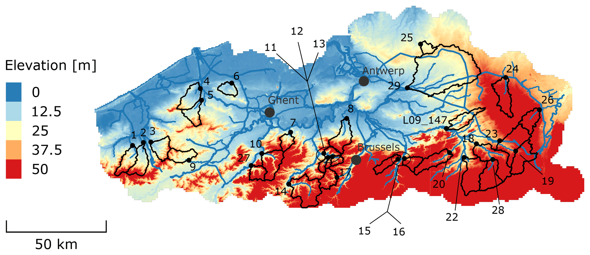
Flanders, with 6.4 million inhabitants, covers around 13 500 km2. The coastal area in the north-west of the region mainly consists of sand dunes and clayey alluvial soils in the polders. The central area mainly consists of loamic soils and ranges between 0 and 10 m. The north-eastern part, known as the Campine region, has sandy soils at altitudes around 30 m. The central southern part with silty soils has low hills up to 150 m. In the south-east, the maximum height is 288 m. The digital terrain model (DTM) in Fig. 1 was taken from the Digital Elevation Model Flanders (“Digitaal Hoogtemodel Vlaanderen”).
Flanders has a maritime climate (Cfb, according to the Köppen climate classification), with average temperatures of 3 and 18 ∘C in January and July, respectively. There is a small gradient present, with lower temperatures in the south-east (annual average of 10 ∘C) towards higher temperatures in the north-west (annual average of 11 ∘C; based on the period 1981 to 2010); the average temperatures in Flanders have increased over the past 30 years by 1 to 1.5 ∘C. Average evapotranspiration was 540 mm year−1 in 1980 and increased almost linearly to 625 mm year−1 in 2010. Yearly precipitation varies between 600 to 1000 mm year−1, with little variation throughout the year and few spatial differences (Brouwers et al., 2015).
Twenty-nine catchments were selected based on a minimum of 20 years of available discharge data. Some of the main characteristics of these catchments are listed in Supplement Table S1. Further, Supplement Figs. S1 and S2 show details of the land cover and soil texture of these catchments, respectively. For land cover, the 30 classes from the ESA CCI Land Cover project were regrouped into the six IPCC land categories, i.e. cropland, forest, grassland, wetland, settlement and other land. This was done in order to reduce the total degrees of freedom for this study. Because the land cover database does not show any significant changes after 2005 (Supplement Fig. S1), the analysis is limited to 1992–2005. Soil texture is obtained from the Flanders underground database; three dominant soil textures (arenic, loamic and silt) cover 99.3 % of the total area of the selected catchments. In this study, only these three dominant soil textures were taken into account.
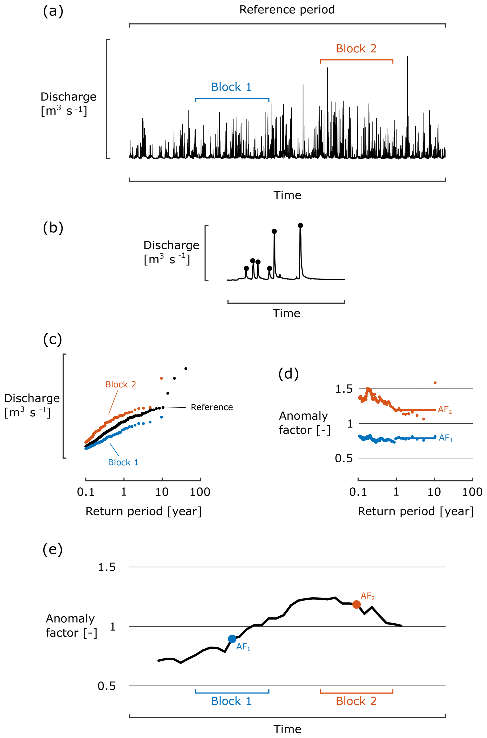
Figure 2Schematic overview of methodology for estimating peak-flow anomalies for two specific block periods over a reference period. (a) Hourly discharge data with indication of two block periods and one reference period; (b) selection of peak flows. (c) Extreme value distribution of peak flows for two block periods and one reference period; (d) anomaly factors for the two block periods as a function of return period and average anomaly factor for return periods larger than 1 year for the two block periods. (e) Average anomaly factors over time, with the average anomaly factors of the two block periods highlighted.
Weather types (see Sect. 3.2) are based on daily mean sea level pressure from the NCEP/NCAR reanalysis data (Kalnay et al., 1996).
The hourly discharge series of each catchment is first transformed to peak-flow anomalies (Sect. 3.1). Then, possible drivers are derived from the data introduced in Sect. 2 and further split into separate categories (see Sect. 3.2). Finally, a regression model is fitted to the data (Sect. 3.3).

Figure 3Regression model combining catchment characteristics, climate variability and land cover changes for explaining streamflow variability.
3.1 Peak-flow anomalies
The methodology for estimating peak-flow anomalies is schematized in Fig. 2. The hourly discharge data (Fig. 2a) is first split into independent events and extremes are extracted (see Fig. 2b) based on a minimum inter-event time and minimum peak values (Willems, 2009). Empirical probabilities (or equivalent return periods) are, on the one hand, assigned to these extremes based on the full time series (reference period), and are, on the other hand, based on subsets of extremes in subperiods and/or blocks of 10 years (Fig. 2c). The quantiles in a particular subperiod and/or block are then compared with the corresponding quantiles based on the reference period, and the ratio of these two empirical quantiles defines an anomaly factor (Fig. 2d). Finally, per subperiod and/or block of 10 years, all anomaly factors corresponding to a return period larger than 1 year are averaged in order to get one value per subperiod of 10 years (Fig. 2d). As such, using a moving window, one can plot and/or investigate peak-flow anomalies for a given catchment over time (Fig. 2e). Note that, when investigating these anomalies over time, a detected signal is only considered robust if it persists for a period longer than the selected block period (here: 10 years). If, for example, an increased anomaly is found for 4 consecutive years and afterwards falls back to the values prior to this increase, this increase is only an artefact of the anomaly method or part of the natural variability.
3.2 Possible drivers
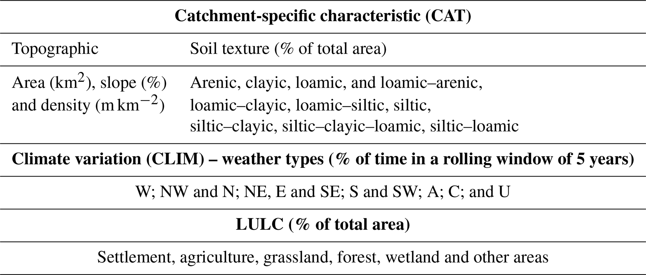
The data introduced in Sect. 2 generally relate to one of the following three categories: catchment-specific characteristics (CATs), climate variations (CLIMs) and land cover (LULCs) changes. Catchment characteristics are considered time invariant in this study and are derived from following sources: the DTM with a spatial resolution of 100 m × 100 m, river map and soil texture. From the DTM and the river map, locations of the outlet stations and catchment delineations are defined. Further, based on the DTM, the slope in the catchment as well as the average slope over the whole catchment are calculated. River density is defined as the ratio of total river length in the catchment to the total area of the catchment. Finally, the relative area of the soil textures are being used in the further analysis. For these soil textures, arenic, loamic and siltic were found to cover 99.3 % of the area of Flanders; when arenic is seen as the complement of loamic and siltic, only two variables remain to describe soil textures. The absence of an explicit variable arenic is compensated through the constant α in the model (see Sect. 3.4.1).
For the weather types, daily mean sea level pressure from the NCEP/NCAR dataset for a 16-point grid around the area of Flanders is used to calculate geostrophic surface flows, shear velocities and flow indices. To convert this into weather types, different classification methods exist (Philipp et al., 2010); here, the Jenkinson–Collison system (Jenkinson and Collison, 1977), a modified version of the Lamb weather-type classification method (Lamb, 1972) is used, distinguishing 28 weather types. These 28 weather types are reduced to 11 by combining all types with the same directional component (see also e.g. Demuzere et al., 2009) and are further reduced based on the link between river peak flows and weather types (De Niel et al., 2017). The remaining groups of weather types are W; NW and N; NE, E and SE; S and SW; U; C; and A, with N, E, S and W referring to wind directions, C and A to cyclonic and anticyclonic atmospheric patterns, respectively, and U referring to an unclassified weather type. This reduction aims to limit the degree of freedom in the final model. In the further analysis, relative frequencies of these daily weather types are considered based on a rolling window of 5 years (Supplement Fig. S3), and U is considered the complement of the other groups of weather types.
Six IPCC land categories (settlement, agriculture, grassland, forest, wetland and other areas) are taken into consideration as possible drivers for this study. It is seen that the maximum proportions of wetland and other areas in the considered catchments are equal to only 0.2 % and 1.5 % respectively. Therefore, these LULC classes will not be further taken into account. In addition, the LULC class grassland is considered as the complement of forest added to agriculture and settlement.
Table 1 summarizes the possible drivers considered in this attribution study.
3.3 Regression model
3.3.1 Panel data analysis
A model is built with the techniques and ideas of panel analysis, which is widely used in social sciences, epidemiology and econometrics where two dimensional data are analysed. Typically, in those sectors data are collected over time and over the same individuals. Here, the two dimensions are space and time; input data can show only a temporal variation (e.g. climate data), only a spatial variation (e.g. soil texture) or a combination of both (e.g. LULC). Note that, typically, climate data show a spatial variation as well. However, in this study, climate variations are described through weather types, and we assume the area of Flanders to be homogeneous with respect to these weather types.
The typical panel data regression model can be described as follows:
with y representing the output of interest, i representing the individual (or catchment) and t representing the time; α and β are constants of dimension 1×1 and 1×n respectively, with n being the number of inputs and/or observations considered. Note that both α and β are catchment independent, as no index i appears here. X represents the input and/or observations as explanatory variables, with dimension (n×1) for each individual (or catchment) at a particular time t, and ϵ is an error term. In this study, the output of interest is the peak-flow anomaly, and inputs can be split into three categories: CATs, CLIMs and LULCs, as described in Table 1. As such, Xit from Eq. (1) becomes:
with superscript T indicating the transpose of a matrix. Next to the linear model (Eq. 1), combined effects of (changes in) observed variables might also play a role in explaining the changes in the output of interest. Therefore, an interaction term is added to the model:
The interaction matrix ρ is of the dimension n×n and is constant, hence being time and catchment independent. This matrix is a strictly upper triangular matrix, meaning that all entries on and below the main diagonal are all equal to 0. Furthermore, for this study, we added the restriction that there cannot be any interaction between explanatory variables from within the same category, for example, .
3.3.2 Model building
Model building happens based on a top-down approach. Starting from a simple constant model, with β=0 and ρ=0, explanatory variables are added to the model based on changes in the value of the Bayesian information criterion (BIC; Kass and Raftery, 1995). BIC is a general criterion for model selection, where models with the lowest BIC are preferred. It takes into account the likelihood of a model, the sample size and the number of parameters estimated by the model. In a first step, only the linear model (Eq. 1) is considered. Once the linear model is fixed, interaction terms are added in a similar way. Note that we only consider interactions between variables present in the linear model. Supposing that βarenic would be equal to 0 in the linear model, then all ρarenic, X in the model including interaction terms are, a priori, set equal to 0.
In order to build a robust model, 100 linear models are tested based on 20 random calibration catchments. Based on this set of 100 models, significant variables are selected, i.e. variables which appear in the majority of the models.
4.1 Final model
The final model has 26 terms in nine predictors (see Supplementary Table S2). During model building, it was decided not to consider the following variables further (Supplement Fig. S4):
-
catchment characteristics, namely area;
-
climate variability in the weather types W; NW and N; NE, E and SE; and U.
The catchment area does not have a significant contribution to the explanation of observed peak-flow changes. Furthermore, when including interaction factors between catchment area and the other variables, model performance did not improve (not shown). This might seem surprising at first, since Blöschl et al. (2007), among others, hypothesize that the land use impact on hydrological response depends on the catchment scale. However, all selected case studies are considered to be of the same scale, despite the differences in catchment area, thus the hypothesized effect of the catchment scale on land use impacts is not applicable here.
One should be careful when interpreting the coefficients from the final model in Supplementary Table S2. For example, the coefficient of Settlement in the final model is equal to −3.04. At first sight, an increase in settlement would thus correspond with a decrease in peak-flow anomaly. However, the interpretation of the coefficients is more complex:
-
An increased settlement area also impacts the interaction effects, and the coefficient becomes .
-
An increased settlement area means that agriculture (13.08) and/or forest (3.71) might decrease; there, again, the interaction effects of agriculture and forest come into play.
The model, as shown in Fig. 3, is able to explain 60 % of the changes in river peak flows over time (Fig. 4). This performance is further broken down into linear effects of the three separate groups and their interactions; linear effects (28 %) are found to be of equal importance as interaction effects (32 %). Within the linear effects, catchment characteristics are most important, as they explain the highest portion (18 %) of the river peak-flow changes, followed by land use and land cover (8 %) and climate variations (6 %). These percentages were obtained by only considering the models that include the variable considered. Note that 18 % + 8 % + 6 % is only slightly larger than 28 %, which is due to a small interdependency between land use and land cover, soil texture, and catchment slope.
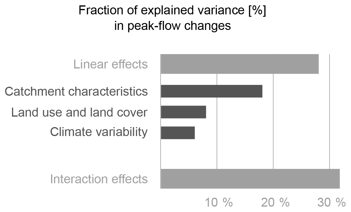
Figure 4Linear effects and interaction effects between catchment characteristics, climate variability and land cover changes play an equal role in explaining streamflow variability.
Observed peak-flow anomalies in catchments 14 (Mark at Viaene) and 17 (Zuunbeek at Sint-Pieters-Leeuw) have a bad correspondence with their modelled results (Fig. 3). Catchment 14 (Mark at Viaene) has a long history of flooding; as of the 2000s, the local authorities have installed several mitigation measures (hydraulic structures, retention basins, etc.), effectively decreasing the flood risk. This is also visible in the observed peak-flow anomaly. However, the regression model used in this study cannot capture such management changes. For catchment 17 (Zuunbeek at Sint-Pieters-Leeuw), increased peak-flow anomalies are observed as from the middle of the period. This is due to the extreme flood season in the winter of 2001–2002, where seven events were observed with peak discharges exceeding 6 m3 s−1 , corresponding to an empirical return period larger than 1 year, based on data between 1978 and 2016.
Ideally, one would carry out a split-sample test (in space and in time) for the estimation of the regression model; however, because of data availability and spatial heterogeneity, this approach would fail in this case. Alternatively, the robustness of the model is tested here by fitting multiple models with different calibration data. It is seen from Fig. 3 that this approach results in consistent estimations for the peak-flow anomalies; only for catchment 26 was this consistency not always found.
4.2 Effect of single drivers
Firstly, the dependency of peak-flow anomalies on catchment characteristics is investigated. This is done by only considering those factors of the model solely consisting of catchment characteristics. It is seen, from Fig. 5, that peak-flow anomalies go up with an increased slope, lower proportion of loamic soil textures and higher proportions of siltic soil textures in the catchments. With respect to river density, the results show less clarity.
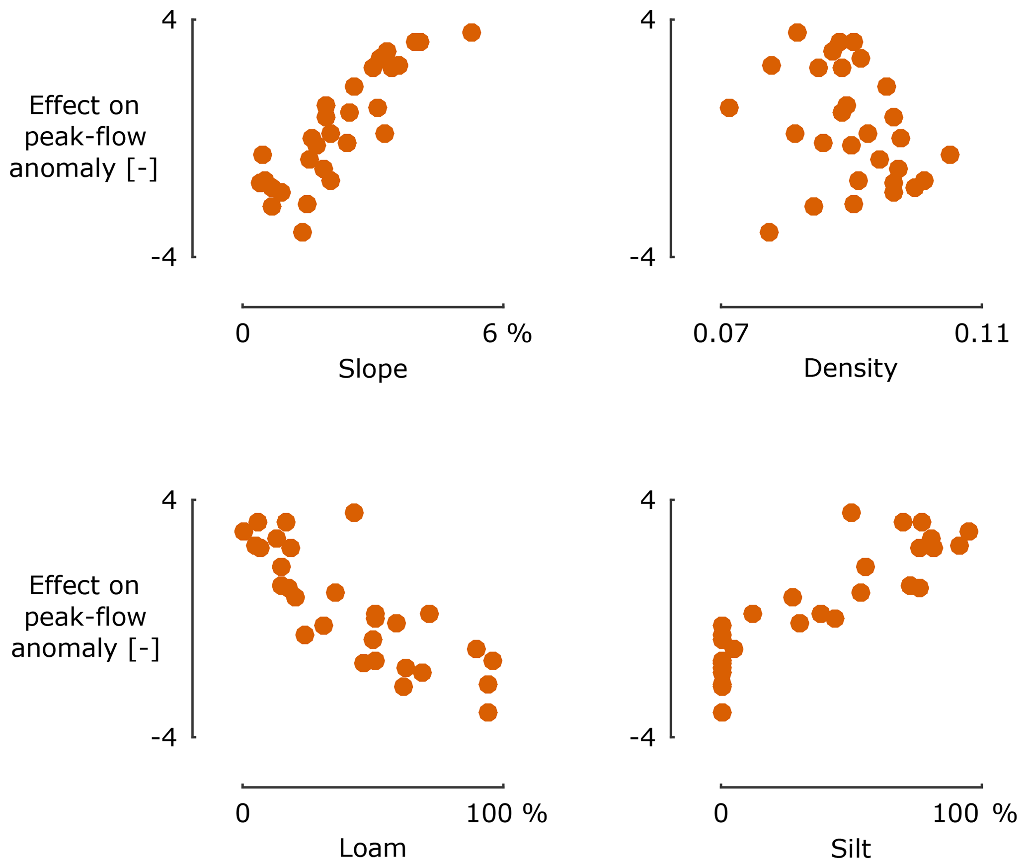
Figure 5Effect of catchment characteristics on peak-flow anomalies for the 29 selected catchments.
These findings correspond to an analysis done on the potential runoff coefficient as used in the hydrological model structure WetSpa (Liu and De Smedt, 2004). The potential runoff coefficient of a catchment is defined as the ratio of runoff volume to rainfall volume. A simple and practical technique was developed in WetSpa to estimate this runoff coefficient as a function of land use, soil texture and slope, based on reference values from literature (Browne, 1990; Chow et al., 1988; Fetter, 1980). See, for example, Fig. 6 for potential runoff coefficients in WetSpa for different combinations of LULC, slope and soil texture. Note that they use slightly different LULC classes, but these differences are insignificant for the purpose of this discussion. From a hydrological point of view and with the above definition of potential runoff coefficient in mind, relative changes in this potential runoff coefficient can serve as a proxy for peak-flow anomalies. As such, findings with respect to the potential runoff coefficient from WetSpa can be related to the conclusions based on Fig. 5:
-
Figure 6a shows that potential runoff coefficients increase with increasing slope. Moreover, the rate of this increase is lower for higher slopes. This corresponds with the findings of this study on catchment slope.
-
Figure 6b and c show that potential runoff coefficients are generally lower for a loamic soil texture compared with a siltic soil texture. This corresponds with the findings of this study on the impact of soil texture classes.
Secondly, with respect to the climate system, it was seen that the relative frequencies of S + SW, combined with the relative frequencies of A, give the most information to the model explaining peak-flow anomalies (Supplement Fig. S4 and Supplement Table S2). This, however, does not mean that the hydrological cycle mostly or only depends on these weather types. Correlations exist between the various weather types; for example frequencies of anticyclonic and cyclonic weather show a negative correlation of −0.79, and frequencies of NW and N have a positive correlation of 0.36. Because of these correlations, we do not make any statements on the effect of increasing or decreasing frequencies of S + SW or A on peak-flow anomalies.

Figure 6Potential runoff coefficient from the WetSpa hydrological model (Liu and De Smedt, 2004) as a function of slope (a) for different LULC categories (loamic soil texture), as a function of soil texture class for different LULC categories (near-zero slope) (b) and as a function of soil texture class for different slopes (forested area; c).
Finally, based on the model, the overall impact of increased urbanization can be investigated. This is done by changing, for each catchment, 1 % of the total area from settlement to forest, grassland and agriculture. This results in increased peak flows for most catchments (Fig. 7), with the disappearing grassland changing to settlement area causing the biggest changes. These results are in line with Hundecha and Bárdossy (2004), who found an increase of 7 % to 10 % in river peak flows for a 15 % increase in urban area at the expense of agricultural land. The strongest changes were found for catchments 1, 2, 3 and 9. These catchments are all quite flat and have a high proportion of loamic soil texture. This finding will further be discussed by investigating the interaction effects below.
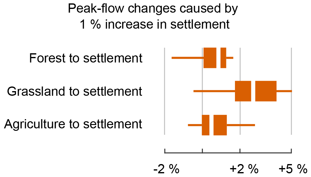
Figure 7Peak-flow changes by increasing settlement area through decreasing forest, grassland or agriculture.
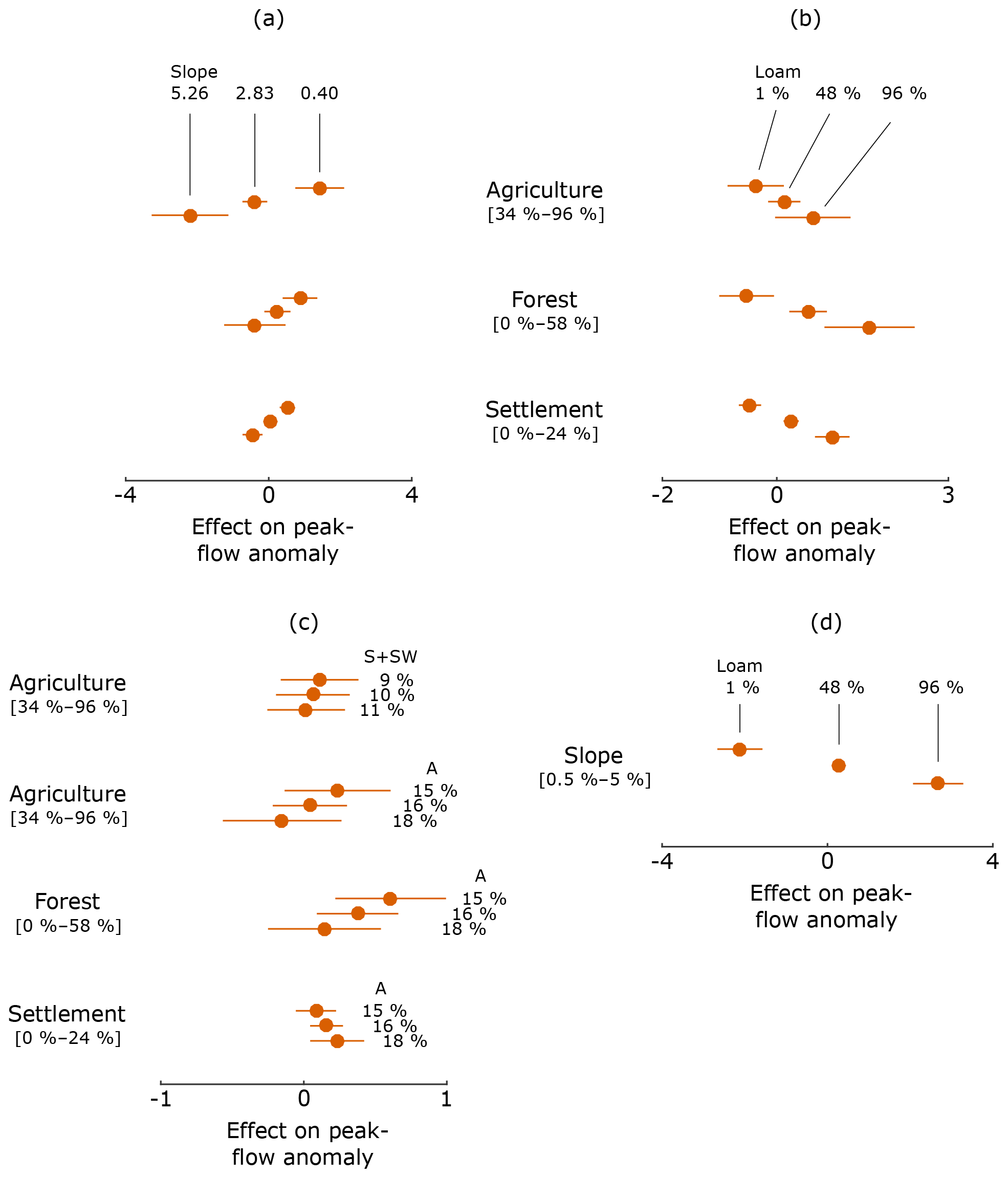
Figure 8Estimated effect on peak-flow anomalies from changing (a) slopes and LULC, (b) soil texture (loamic content) and LULC, (c) climatic conditions (relative frequencies of weather types S + SW and A) and LULC, and (d) slopes and soil texture (loamic content), averaging out the effects of the other predictors. Horizontal bars indicate confidence intervals for the estimated effect.
4.3 Interaction effects
The total number of interaction effects (32 %) is largely carried by three terms only, namely interaction between LULC and soil texture classes (% loamic; 10 %), between LULC and slope (6 %), and between soil texture classes (% loamic) and slope (6 %; see Fig. 8):
-
Figure 8a shows effects of LULC changes on peak-flow anomalies as a function of the slope (three particular slopes are shown: flat– 0.40, medium – 2.83 – and steep – 5.26). Note that this graph was obtained by averaging out effects of other predictors, and, as such, the absolutes values of the effects should be interpreted carefully. For the purpose of interaction effects, results of Fig. 8 should be interpreted in a relative way. It is seen that, with an increasing slope, the effect of LULC changes on peak-flow anomaly goes down. A steeper slope typically results in increased peak flows, but the LULC changes influence these peak-flow anomalies to a lesser degree compared with more flat catchments. Note that, although different in magnitude, these trends are consistent for each LULC class.
-
Similar to the interaction between slope and LULC, catchments with a low proportion of loamic soil textures are less influenced by LULC changes with respect to peak-flow anomalies compared with catchments with a high proportion of loamic soils (Fig. 8b). Again, trends are consistent for each LULC class.
-
And finally, the catchment slope has a larger effect with respect to peak-flow anomalies in catchments with a high proportion on loamic soil textures compared with a catchment with a lower proportion on loamic soil textures (Fig. 8d).
Comparison with the analysis on the potential runoff coefficient from WetSpa (Fig. 6) results in the following three main interaction effects:
-
Slope and LULC. One can see in Fig. 6a that the range of potential runoff coefficients between the four LULC classes is significantly larger at a near-zero slope compared with a slope of 100 %. In other words, relative changes in the potential runoff coefficient with changing LULC are smaller for catchments with a steeper slope.
-
Soil texture and LULC. For catchments with a pure loamic soil texture, the potential runoff coefficient at a near-zero slope increases by a factor 4.4 from a forested area (0.14) to a mixed urban area (0.62). For catchments with a pure siltic soil texture (thus, with a very low contribution of loamic), this is only a factor of 3.1 (0.21 vs. 0.66; Fig. 6b). In other words, loamic catchments are more sensitive to LULC changes with respect to potential runoff coefficients.
-
Soil texture and slope. For catchments with a pure loamic soil texture, the potential runoff coefficient in forested area increases by 42 % between a slope of 1 % (0.14) and 5 % (0.20). For catchments with a pure siltic soil texture (thus, with a very low contribution of loamic), this is only 29 % (0.21 vs. 0.27; Fig. 6c). In other words, loamic catchments are more sensitive to the catchment slope with respect to potential runoff coefficients.
Interaction terms between LULC and climatic conditions holds only 2 % of explanatory power in the models. Figure 8c shows these minor interactions. Periods in time with many anticyclonic weather types show a decreased sensitivity to changes in agricultural and forested land and an increased sensitivity to settlement area. Moreover, a decreased sensitivity to agricultural land is seen for periods with many S and SW weather types. However, since the confidence intervals for the different climatic conditions overlap in all four cases of Fig. 8c, these interactions might not be significant.
The remaining interaction terms (Supplement Table S2) further explain an additional 8 % of the variation in peak-flow anomalies. Note that no significant interaction terms were found between catchment characteristics and climate conditions. This would mean that each catchment responds in a similar way to climatic oscillations.
The regression model is able to explain 60 % of the changes in peak-flow extremes. For catchments 14 (Mark at Viaene) and 17 (Zuunbeek at Sint-Pieters-Leeuw), however, the model is not able to mimic observed step changes. For the other 27 considered catchments, the direction and the overall trends simulated by the model are found to be accurate.
It was seen that for these case studies, changes in land cover and climate variations play an equally important role in explaining changes in river peak flows. These effects, however, are of a lower importance than catchment specific factors, such as topography and soil texture; higher peak flow can be expected for catchments with a high average slope, a low proportion of loamic soil texture and high proportion of siltic soil. The high importance of these time-invariant factors (topography and soil texture) indicate that flood response in Flanders is highly catchment specific and, to a lesser degree, depends on fluctuations of the climate and land use changes.
Obviously, given the complexity of these environmental systems, the simple linear model will not be able to capture and/or describe all effects; indeed, it was seen that interaction effects between catchment characteristics, land cover and climate variations are equally important in explaining changes in river peak flows. It was shown that the sensitivity with respect to peak-flow changes caused by LULC changes is lower for catchments with a steep slope and a low proportion of loamic soil textures. The model also showed that, for most of the considered catchments in this study, the effect of a decrease in forested area to an increase in settlement area indeed leads to increased peak flows. Moreover, a 1 % increase in settlement could lead in some cases to a 5 % increase in river peak flows. These results provide important new findings to support urban planning and flood management. Firstly, the link between slope, soil texture and peak flows can help in developing catchment-specific flood management plans. Also, the land use changes should be planned taking catchment characteristics into account, since it was shown that land use change impacts on peak flows differ significantly in catchments with different slopes and soil textures.
All data were obtained via publicly available sources. The DTM was obtained from the “Digitaal Hoogtemodel Vlaanderen” (VMM, Watlab and Agiv), available from https://download.vlaanderen.be/Producten/Detail?id=1485&title=Digitaal_Hoogtemodel_Vlaanderen_II_DTM_raster_100_m (VMM, Watlab and AGIV (Belgium), 2016). The river network and catchment delineation was obtained from the “Vlaamse Hydrografische Atlas” (http://www.geopunt.be/catalogus/datasetfolder/295615a5-3104-47b3-b8d4-9bbeb23b53ea, AGIV (Belgium), 2016). Land cover was obtained from the ESA CCI Land Cover project (http://maps.elie.ucl.ac.be/CCI/viewer/, ESA CCI Land Cover project, 2018). Soil texture data are available on https://www.dov.vlaanderen.be/geonetwork/apps/tabsearch/index.html?uuid=83c46eae-a202-454c-b063-a858be3e4335 (Vlaamse overheid, Departement Omgeving, Vlaams Planbureau voor Omgeving (VPO), 2018). The NCEP/NCAR reanalysis data were provided by the NOAA/OAR/ESRL PSD in Boulder, Colorado, USA, from their website at https://www.esrl.noaa.gov/psd/data/gridded/data.ncep.reanalysis.html (NOAA/OAR/ESRL PSD, 2018). The discharge data were obtained from https://www.waterinfo.be/default.aspx?path=NL/Rapporten/Downloaden (Waterinfo.be, 2018).
The supplement related to this article is available online at: https://doi.org/10.5194/hess-23-871-2019-supplement.
JDN and PW worked on the conceptualization of the research and jointly developed the methodology. JDN curated the data and performed the formal analysis and investigation, under the supervision of PW. JDN prepared the visualization and the initial draft, which was critically reviewed and revised by PW.
The authors would like to thank colleague Els Van Uytven from KU Leuven for
deriving the weather types. Also, the organizations VMM, Watlab, Agiv, ESA
and NOAA are gratefully acknowledged for making their data publicly
available. We would also like to thank Woonsup Choi and two other anonymous reviewers and the
editor, whose comments and suggestions helped improve and clarify this
paper.
Edited by: Nadav Peleg
Reviewed by: Woonsup Choi and two anonymous referees
AGIV (Belgium): Vlaamse Hydrografische Atlas, available at: http://www.geopunt.be/catalogus/datasetfolder/295615a5-3104-47b3-b8d4-9bbeb23b53ea, last access: 6 January 2017.
Blöschl, G., Ardoin-Bardin, S., Bonell, M., Dorninger, M., Goodrich, D., Gutknecht, D., Matamoros, D., Merz, B., Shand, P., and Szolgay, J.: At what scales do climate variability and land cover change impact on flooding and low flows?, Hydrol. Process., 1247, 1241–1247, https://doi.org/10.1002/hyp.6669, 2007.
Brisson, E., Demuzere, M., Kwakernaak, B., and Van Lipzig, N. P. M.: Relations between atmospheric circulation and precipitation in Belgium, Meteorol. Atmos. Phys., 111, 27–39, https://doi.org/10.1007/s00703-010-0103-y, 2011.
Bronstert, A., Niehoff, D., and Brger, G.: Effects of climate and land-use change on storm runoff generation: Present knowledge and modelling capabilities, Hydrol. Process., 16, 509–529, https://doi.org/10.1002/hyp.326, 2002.
Brouwers, J., Peeters, B., Van Steertegem, M., van Lipzig, N., Wouters, H., Beullens, J., Demuzere, M., Willems, P., De Ridder, K., Maiheu, B., De Troch, R., Termonia, P., Vansteenkiste, Th., Craninx, M., Maetens, W., Defloor, W., and Cauwenberghs, K.: MIRA Klimaatrapport 2015, over waargenomen en toekomstige klimaatveranderingen. Vlaamse Milieumaatschappij in cooperation with KU Leuven, VITO and KMI. Aalst, Belgium, 147 p., available at: https://www.milieurapport.be/publicaties/2015/klimaatrapport-2015-over-waargenomen-en-toekomstige-klimaatveranderingen (last access: 12 July 2018), 2015.
Browne, F. X.: Stormwater Management, in: Standard Handbook of Environmental Engineering, edited by: Corbitt, R. A., McGraw-Hill, New York, 1990.
Chow, V. T., Maidment, D. R., and Mays, L. W.: Applied Hydrology, McGraw-Hill, New York, 1988.
Demuzere, M., Werner, M., van Lipzig, N., and Roeckner, E.: An analysis of present and future ECHAM5 pressure fields using a classification of circulation patterns, Int. J. Climatol., 29, 1796–1810, 2009.
De Niel, J., Demarée, G., and Willems, P.: Weather Typing-Based Flood Frequency Analysis Verified for Exceptional Historical Events of Past 500 Years Along the Meuse River, Water Resour. Res., 53, 8459–8474, https://doi.org/10.1002/2017WR020803, 2017.
Dey, P. and Mishra, A.: Separating the impacts of climate change and human activities on streamflow: A review of methodologies and critical assumptions, J. Hydrol., 548, 278–290, https://doi.org/10.1016/j.jhydrol.2017.03.014, 2017.
ESA CCI Land Cover project: Land Cover Map 2015, UCLouvain (Belgium), available at: http://maps.elie.ucl.ac.be/CCI/viewer/, last access: 23 January 2018.
Fetter, C. W.: Applied Hydrogeology, C. E. Merril, Columbus, 1980.
Galster, J. C., Pazzaglia, F. J., Hargreaves, B. R., Morris, D. P., Peters, S. C., and Weisman, R. N.: Effects of urbanization on watershed hydrology: The scaling of discharge with drainage area, Geology, 34, 713, https://doi.org/10.1130/G22633.1, 2006.
Hall, J., Arheimer, B., Borga, M., Brázdil, R., Claps, P., Kiss, A., Kjeldsen, T. R., Kriauciuniene, J., Kundzewicz, Z. W., Lang, M., Llasat, M. C., Macdonald, N., McIntyre, N., Mediero, L., Merz, B., Merz, R., Molnar, P., Montanari, A., Neuhold, C., Parajka, J., Perdigão, R. A. P., Plavcová, L., Rogger, M., Salinas, J. L., Sauquet, E., Schär, C., Szolgay, J., Viglione, A., and Blöschl, G.: Understanding flood regime changes in Europe: a state-of-the-art assessment, Hydrol. Earth Syst. Sci., 18, 2735–2772, https://doi.org/10.5194/hess-18-2735-2014, 2014.
Hamdi, R., Termonia, P., and Baguis, P.: Effects of urbanization and climate change on surface runoff of the Brussels Capital Region: A case study using an urban soil-vegetation-atmosphere-transfer model, Int. J. Climatol., 31, 1959–1974, https://doi.org/10.1002/joc.2207, 2011.
Hegerl, G. C., Hoegh-Guldberg, O., Casassa, G., Hoerling, M. P., Kovats, R. S., Parmesan, C., Pierce, D. W., and Stott, P. A.: Good Practice Guidance Paper on Detection and Attribution Related to Anthropogenic Climate Change, in: Meeting Report of the Intergovernmental Panel on Climate Change Expert Meeting on Detection and Attribution of Anthropogenic Climate Change, edited by: Stocker, T. F., Field, C. B., Qin, D., Barros, V., Plattner, G.-K., Tignor, M., Midgley, P. M., and Ebi, K. L., p. 8, IPCC Working Group I Technical Support Unit, University of Bern, Bern, Switzerland, 2010.
Hirschboek, K. K.: Climate and Floods, US Geol. Surv. Water-Supply Pap., 2375, 67–88, 1991.
Hundecha, Y. and Bárdossy, A.: Modeling of the effect of land use changes on the runoff generation of a river basin through parameter regionalization of a watershed model, J. Hydrol., 292, 281–295, https://doi.org/10.1016/J.JHYDROL.2004.01.002, 2004.
IPCC: Climate Change 2014: Synthesis Report. Contribution of Working Groups I, II and III to the Fifth Assessment Report of the Intergovernmental Panel on Climate Change, edited by: Core Writing Team, Pachauri, R. K., and Meyer, L. A., IPCC, Geneva, Switzerland, 2014.
Jenkinson, A. F. and Collison, B. P.: An Initial Climatology of Gales Over the North Sea, Bracknell, UK, 1977.
Kalnay, E., Kanamitsu, M., Kistler, R., Collins, W., Deaven, D., Gandin, L., Iredell, M., Saha, S., White, G., Woollen, J., Zhu, Y., Chelliah, M., Ebisuzaki, W., Higgins, W., Janowiak, J., Mo, K. C., Ropelewski, C., Wang, J., Leetmaa, A., Reynolds, R., Jenne, R., and Joseph, D.: The NCEP/NCAR 40-Year Reanalysis Project, B. Am. Meteorol. Soc., 77, 437–470, 1996.
Kass, R. E. and Raftery, A. E.: Bayes Factors, J. Am. Stat. Assoc., 90, 773–795, 1995.
Lamb, H. H.: British isles weather types and a register of daily sequence of circulation patterns, 1861–1971, Geophysical Memoir 116, HMSO, London, 85 pp., 1972.
Liu, Y. and De Smedt, F.: WetSpa Extension, Documentation and User Manual, Department of Hydrology and Hydraulic Engineering, Vrije Universiteit Brussel, 2004.
Mediero, L., Kjeldsen, T. R., Macdonald, N., Kohnova, S., Merz, B., Vorogushyn, S., Wilson, D., Alburquerque, T., Blöschl, G., Bogdanowicz, E., Castellarin, A., Hall, J., Kobold, M., Kriauciuniene, J., Lang, M., Madsen, H., Onuşluel Gül, G., Perdigão, R. A. P., Roald, L. A., Salinas, J. L., Toumazis, A. D., Veijalainen, N., and Þórarinsson, Ó.: Identification of coherent flood regions across Europe by using the longest streamflow records, J. Hydrol., 528, 341–360, https://doi.org/10.1016/j.jhydrol.2015.06.016, 2015.
Merz, B., Vorogushyn, S., Uhlemann, S., Delgado, J., and Hundecha, Y.: HESS Opinions “More efforts and scientific rigour are needed to attribute trends in flood time series”, Hydrol. Earth Syst. Sci., 16, 1379–1387, https://doi.org/10.5194/hess-16-1379-2012, 2012.
NOAA/OAR/ESRL PSD (Colorado, USA): NCEP/NCAR Reanalysis 1: Summary, available at: https://www.esrl.noaa.gov/psd/data/gridded/data.ncep.reanalysis.html, last access: 19 January 2018.
Pfister, L., Kwadijk, J., Musy, A., Bronstert, A., and Hoffmann, L.: Climate change, land use change and runoff prediction in the Rhine-Meuse basins, River Res. Appl., 20, 229–241, https://doi.org/10.1002/rra.775, 2004.
Philipp, A., Bartholy, J., Beck, C., Erpicum, M., Esteban, P., Fettweis, X., Huth, R., James, P., Jourdain, S., Kreienkamp, F., Krennert, T., Lykoudis, S., Michalides, S. C., Pianko-Kluczynska, K., Post, P., Álvarez, D. R., Schiemann, R., Spekat, A., and Tymvios, F. S.: Cost733cat – A database of weather and circulation type classifications, Phys. Chem. Earth, 35, 360–373, https://doi.org/10.1016/j.pce.2009.12.010, 2010.
Poelmans, L.: Modelling urban expansion and its hydrological impacts, KU Leuven (University of Leuven), 2010.
Poelmans, L., Rompaey, A. Van, Ntegeka, V., and Willems, P.: The relative impact of climate change and urban expansion on peak flows: a case study in central Belgium, Hydrol. Process., 25, 2846–2858, https://doi.org/10.1002/hyp.8047, 2011.
Prudhomme, C. and Genevier, M.: Can atmospheric circulation be linked to flooding in Europe?, Hydrol. Process., 25, 1180–1190, https://doi.org/10.1002/hyp.7879, 2011.
Ruimte Vlaanderen: Witboek Beleidsplan Ruimte Vlaanderen, Brussels, Belgium, available at: https://www.ruimtevlaanderen.be/brv (last access: 12 July 2018), 2017.
Smith, J. A., Villarini, G., and Baeck, M. L.: Mixture Distributions and the Hydroclimatology of Extreme Rainfall and Flooding in the Eastern United States, J. Hydrometeorol., 12, 294–309, https://doi.org/10.1175/2010JHM1242.1, 2011.
Tabari, H., Taye, M. T., and Willems, P.: Water availability change in central Belgium for the late 21st century, Glob. Planet. Change, 131, 115–123, https://doi.org/10.1016/j.gloplacha.2015.05.012, 2015.
Tavakoli, M., De Smedt, F., Vansteenkiste, T., and Willems, P.: Impact of climate change and urban development on extreme flows in the Grote Nete watershed, Belgium, Nat. Hazards, 71, 2127–2142, https://doi.org/10.1007/s11069-013-1001-7, 2014.
Tu, M., Hall, M. J., de Laat, P. J. M., and de Wit, M. J. M.: Extreme floods in the Meuse river over the past century: Aggravated by land-use changes?, Phys. Chem. Earth, 30(4–5 SPEC. ISS.), 267–276, https://doi.org/10.1016/j.pce.2004.10.001, 2005.
United Nations: World Urbanization Prospects: The 2018 Revision, Online Edition, available at: https://esa.un.org/unpd/wup/, last access: 12 July 2018.
Van Loon, A. F., Stahl, K., Di Baldassarre, G., Clark, J., Rangecroft, S., Wanders, N., Gleeson, T., Van Dijk, A. I. J. M., Tallaksen, L. M., Hannaford, J., Uijlenhoet, R., Teuling, A. J., Hannah, D. M., Sheffield, J., Svoboda, M., Verbeiren, B., Wagener, T., and Van Lanen, H. A. J.: Drought in a human-modified world: reframing drought definitions, understanding, and analysis approaches, Hydrol. Earth Syst. Sci., 20, 3631–3650, https://doi.org/10.5194/hess-20-3631-2016, 2016.
Vansteenkiste, T., Tavakoli, M., Van Steenbergen, N., De Smedt, F., Batelaan, O., Pereira, F., and Willems, P.: Intercomparison of five lumped and distributed models for catchment runoff and extreme flow simulation, J. Hydrol., 511, 335–349, https://doi.org/10.1016/j.jhydrol.2014.01.050, 2014.
Vlaamse overheid, Departement Omgeving, Vlaams Planbureau voor Omgeving (VPO): WRB Soil Units 40k: Bodemkaart van het Vlaamse Gewest volgens het internationale bodemclassificatiesysteem World Reference Base op schaal 1 : 40.000, available at: https://www.dov.vlaanderen.be/geonetwork/apps/tabsearch/index.html?uuid=83c46eae-a202-454c-b063-a858be3e4335, last access: 29 January 2018.
VMM, Watlab and AGIV (Belgium): Digitaal Hoogtemodel Vlaanderen, available at: https://download.vlaanderen.be/Producten/Detail?id=1485&title=Digitaal_Hoogtemodel_Vlaanderen_II_DTM_raster_100_m, last access: 9 August 2016.
Waterinfo.be: Discharge data, available at: https://www.waterinfo.be/default.aspx?path=NL/Rapporten/Downloaden, last access: 11 January 2018.
Willems, P.: A time series tool to support the multi-criteria performance evaluation of rainfall-runoff models, Environ. Model. Softw., 24, 311–321, https://doi.org/10.1016/j.envsoft.2008.09.005, 2009.
Willems, P.: Multidecadal oscillatory behaviour of rainfall extremes in Europe, Clim. Change, 120, 931–944, https://doi.org/10.1007/s10584-013-0837-x, 2013.
Zhang, M., Liu, N., Harper, R., Li, Q., Liu, K., Wei, X., Ning, D., Hou, Y., and Liu, S.: A global review on hydrological responses to forest change across multiple spatial scales: Importance of scale, climate, forest type and hydrological regime, J. Hydrol., 546, 44–59, https://doi.org/10.1016/j.jhydrol.2016.12.040, 2017.