the Creative Commons Attribution 4.0 License.
the Creative Commons Attribution 4.0 License.
 | 04 Mar 2020
Calibration of hydrological models for ecologically relevant streamflow predictions: a trade-off between fitting well to data and estimating consistent parameter sets?
Thibault Hallouin
Michael Bruen
Fiachra E. O'Loughlin
The ecological integrity of freshwater ecosystems is intimately linked to natural fluctuations in the river flow regime. In catchments with little human-induced alterations of the flow regime (e.g. abstractions and regulations), existing hydrological models can be used to predict changes in the local flow regime to assess any changes in its rivers' living environment for endemic species. However, hydrological models are traditionally calibrated to give a good general fit to observed hydrographs, e.g. using criteria such as the Nash–Sutcliffe efficiency (NSE) or the Kling–Gupta efficiency (KGE). Much ecological research has shown that aquatic species respond to a range of specific characteristics of the hydrograph, including magnitude, frequency, duration, timing, and the rate of change of flow events. This study investigates the performance of specially developed and tailored criteria formed from combinations of those specific streamflow characteristics (SFCs) found to be ecologically relevant in previous ecohydrological studies. These are compared with the more traditional Kling–Gupta criterion for 33 Irish catchments. A split-sample test with a rolling window is applied to reduce the influence on the conclusions of differences between the calibration and evaluation periods. These tailored criteria are shown to be marginally better suited to predicting the targeted streamflow characteristics; however, traditional criteria are more robust and produce more consistent behavioural parameter sets, suggesting a trade-off between model performance and model parameter consistency when predicting specific streamflow characteristics. Analysis of the fitting to each of 165 streamflow characteristics revealed a general lack of versatility for criteria with a strong focus on low-flow conditions, especially in predicting high-flow conditions. On the other hand, the Kling–Gupta efficiency applied to the square root of flow values performs as well as two sets of tailored criteria across the 165 streamflow characteristics. These findings suggest that traditional composite criteria such as the Kling–Gupta efficiency may still be preferable over tailored criteria for the prediction of streamflow characteristics, when robustness and consistency are important.
- Article
(3128 KB) -
Supplement
(155 KB) - BibTeX
- EndNote


River flow is the cornerstone of freshwater ecosystems, the ecological integrity of which relies on natural fluctuations in the river flow regime (Poff et al., 1997). A long history of human alterations of the river flow regime for water supply, irrigation, flood protection, or hydropower threatens water security and freshwater biodiversity in many regions of the world (Vörösmarty et al., 2010). Richter et al. (1997) raised the overarching research question: “How much water does a river need?”. In order to quantify these needs and assess the effects of altered flow regime on freshwater ecology, many different hydrological indices have been used, whether they are referred to as streamflow characteristics (SFCs) (Vis et al., 2015; Pool et al., 2017), ecologically relevant flow statistics (ERFSs) (Caldwell et al., 2015), or indicators of hydrological alteration (IHAs) (Richter et al., 1996). These SFCs describe specific aspects of the river flow regime that can be extracted from the streamflow hydrograph and can be categorised on the basis of magnitude, frequency, rate of change, timing, and duration of high-, average-, and low-flow events (Poff et al., 1997). Olden and Poff (2003) listed a range of such SFCs used to characterise river flow regime in relation to ecological species' preferences. The prediction of these SFCs at ungauged locations has historically been done using statistical analyses such as regional regression models that relate them to some climatic and physiographic descriptors (e.g. Carlisle et al., 2011; Knight et al., 2014). However, these regression models are not well-suited for investigating water management or climate change scenarios because they often rely on long-term descriptors, assumed to be stationary. On the other hand, hydrological models can allow for such scenario analyses, and they produce simulated streamflow hydrographs from which the streamflow characteristics can be computed (e.g. Shrestha et al., 2014; Caldwell et al., 2015).
Most rainfall–runoff models used to predict SFCs relevant for stream ecology require parameter calibration. The selection of the calibration criterion or objective function is of great importance for predictions of SFCs (Vis et al., 2015; Kiesel et al., 2017; Pool et al., 2017). As demonstrated by Vis et al. (2015), different sets of parameters, each equally well-performing based on the Nash–Sutcliffe efficiency (NSE) criterion (Nash and Sutcliffe, 1970), can yield very different performances when looking at the prediction of SFCs. This exposes the limitations of models in representing the entirety of real-world processes in a catchment. Indeed, because of uncertainties in model structure, model forcing, and evaluation data (Beven, 2016), the identification of a single perfect parameter set is usually unachievable (Beven, 2006), and in practice trade-offs are required between modelling different aspects of the hydrograph. The choice of the objective function directly influences which trade-offs are made. The calibration of a rainfall–runoff model using the NSE gives more importance to fitting flow peaks because of its quadratic formulation, and this is reflected in its better performance in general in predicting streamflow characteristics for high-flow conditions (Shrestha et al., 2014). Composite objective functions such as the Kling–Gupta efficiency (KGE) are now often preferred, since KGE explicitly considers linear correlation, bias, and variability in a balanced or customisable way (Gupta et al., 2009; Kling et al., 2012). Nonetheless, the quadratic formulation based on flows remains in the linear correlation component of KGE, and a prior transformation of flow values is often suggested, for example to put more emphasis on low flows (Santos et al., 2018). In order to improve the model calibration for the predictions of the entire hydrograph, the whole or parts of the flow duration curve have also been found useful (e.g. Westerberg et al., 2011; Pfannerstill et al., 2014). However, the flow duration curve does not embed any information about the timing or duration of flow events, which can be essential for some species (Arthington et al., 2006).
In order to improve the prediction of a diverse range of SFCs (e.g. related to both high-flow and low-flow conditions or both magnitude and duration of flows), multi-objective calibration methods applied to flows (referred to as traditional objective functions hereafter) have been explored by others. For instance, Vis et al. (2015) found that certain combinations of objective functions each focussing on different statistical aspects of the hydrograph tend to be more suitable for the prediction of the magnitude of average flows and the timing of moderate and low flows than using a single objective function. But on average, they found that NSE calibration produces the smallest errors for 12 SFCs, and they did not find a single best calibration strategy for predicting all SFCs at once. Garcia et al. (2017) identified that an average of KGE applied to flows and KGE applied to inverted flows has a better skill at predicting seven SFCs relative to low-flow conditions than either normal KGE or KGE applied to inverted flows alone. Hernandez-Suarez et al. (2018) found that a three-criteria calibration strategy with NSE, NSE of the square root transformed flows, and NSE on the relative deviations can predict 128 SFCs within a ±30 % error range in their study catchment, with larger errors on SFCs for extreme high- and low-flow conditions. Mizukami et al. (2019) compared objective functions that predict the bias in annual peak flows, and they found that KGE was better suited than NSE at reproducing the flow variability, reducing, but not eliminating, the underestimation of high flows. These studies suggest that combinations of traditional objective functions (e.g. NSE and KGE) on transformed and untransformed streamflow series can improve the prediction of SFCs compared to single objective calibration strategies, while the predictions of extreme flow conditions remain problematic.
To further improve the prediction of a range of SFCs, a pragmatic approach is to use an objective function fitted to the target SFCs (referred to as tailored objective functions hereafter) in the expectation that this will improve predictions of these same SFCs. Mizukami et al. (2019) found that the annual peak flow bias was best predicted by using the bias itself as the objective function (to be minimised), outperforming KGE, and other KGE formulations that had more weight on flow variability, but they also found that using this single SFC as an objective function resulted in overfitting, reducing its transferability in time. Pool et al. (2017) also found that a given SFC is the best objective function for a model intended to predict itself, and, for 13 different SFCs, this approach outperformed NSE. The authors also used a four-SFC metric as the objective function, but the prediction of other SFCs, not included in this objective function, was not improved compared to NSE. Kiesel et al. (2017) used a seven-SFC metric as objective function to predict seven SFCs, and they found that this objective function outperformed KGE on almost all seven SFCs. The authors also found that for two of these seven, SFCs used as a single objective function produced better overall performance than KGE. Zhang et al. (2016) found that a 16-SFC metric used as the objective function outperformed the RMSE, especially for the prediction of SFCs based on low- and high-flow events. On the other hand, Garcia et al. (2017) reached a different conclusion when predicting seven SFCs focussing on low-flow conditions, where their combined seven-SFC metric was not as robust as the composite objective function made of KGE and KGE on inverted flows. However, unlike the other studies previously mentioned, this multi-SFC metric focussed solely on low-flow conditions, which could explain its lack of robustness, given its difficulty in predicting extreme flows well.
Hydrological models are generally found to be less accurate than regional regression models in predicting particular SFCs because separate regression models can be developed for each target SFC (Murphy et al., 2013). Similar behaviour has been found for calibrated rainfall–runoff models, where specific calibration focussed on the target SFC is the best calibration option for predicting that SFC (Kiesel et al., 2017; Pool et al., 2017; Mizukami et al., 2019). However, while calibrating on a specific SFC may improve the model's ability to predict that indicator, its representation of the catchment's overall behaviour could be compromised, limiting the value of the model for predicting other indicators. For instance, Pool et al. (2017) found that using a combination of SFCs as an objective function does not perform as well as the Nash–Sutcliffe efficiency fitted to flows to predict SFCs not included in the calibration, and the authors suggested that the use of SFCs in calibration may not produce consistent model parameter sets. Poff and Zimmerman (2010) and Knight et al. (2014) showed that each aquatic species is sensitive to its own combination of SFCs relating to its own preferences for living conditions (Knight et al., 2012). When several species are considered simultaneously, the number of SFCs to predict is likely to increase, even though some species may respond to broadly similar streamflow characteristics. If the number of SFCs to predict were to increase, it could be expected that using traditional objective functions would be a more parsimonious calibration strategy and that more targeted characteristics of the hydrograph would be predicted well. For example, Archfield et al. (2014) found that a set of seven streamflow statistics based on daily streamflows, including traditional objective functions fitted to flows, is more parsimonious than a set of 33 SFCs to classify stream gauges for hydro-ecological purposes.
The objectives of this study are to compare the skills of tailored objective functions fitted to SFCs against more traditional objective functions fitted to flows to predict SFCs. This comparison is articulated around four research questions:
- Q1
Which objective function provides the most accurate SFC predictions?
- Q2
Which objective function provides the most robust SFC predictions?
- Q3
Which objective function provides the most stable SFC predictions?
- Q4
Which objective function yields the most consistent behavioural parameter sets?
In order to consider the notions of stability and consistency, 14 different calibration–evaluation periods are used. Moreover, three different sets of SFCs are considered as prediction targets in order to overcome the possibility of the conclusions being specific to the combinations of SFCs considered. In addition, the skill of the objective functions are compared on a set of 156 SFCs and on 9 percentiles of the flow duration curve to extend the comparison beyond the SFCs contained in the tailored objective functions and explore trends on specific categories of streamflow characteristics.
The paper is organised as follows: Sect. 2 describes the data and models used for the study; Sect. 3 unveils the methodology employed to answer the research questions above; Sect. 4 presents the results of the comparison of the objective functions; and Sect. 5 draws on the findings and their implications for the predictions of SFCs and discusses the limitations of the study.
2.1 Streamflow characteristics
In the absence of adequate local data, the selection of streamflow characteristics used in the tailored objective functions relies on previous studies that identified sets of SFCs representative of the habitat preferences of fish communities in the southeastern US (Knight et al., 2014; Pool et al., 2017) and of invertebrate communities in Germany (Kakouei et al., 2017; Kiesel et al., 2017). In addition, a third set of SFCs is formed by combining the first two sets of SFCs, assuming that invertebrate and fish communities are sensitive to two mainly distinct habitat preferences, requiring a larger set of SFCs. These three sets are assumed to be of some ecological relevance to the Irish study catchments for the purpose of comparing traditional and plausible tailored objective functions; however, currently there is a scarcity of direct empirical evidence to confirm this.
The indices are listed and detailed in Table 1. Except for q85 that is derived from the flow duration curve, all streamflow characteristics are defined in Olden and Poff (2003) and their calculation follows the method implemented in the R package EflowStats (Henriksen et al., 2006; Archfield et al., 2014). However, all computations for this study were carried out in Python where the NumPy package was used to vectorise the calculations of the SFCs (i.e. to formulate the calculations as arithmetic operations between vectors and matrices) (Hallouin, 2019a).
Table 1List and description of the 18 selected streamflow characteristics. Detailed calculations for each SFC available in Table . The three last columns indicate whether a given SFC is included (∈) or not included (∉) in Eq. (4) for the definition of each of the three tailored objective functions.

2.2 Study catchments
This study used discharge records with a minimum of 14 hydrological years with complete daily discharge data in the period from 1 October 1986 to 30 September 2016. If any daily value was missing, the relevant hydrological year was discarded as the calculation of some streamflow characteristics requires a strictly continuous daily streamflow time series. The length of 14 years was set as the minimum requirement in order to have 7 years for calibration and 7 years for evaluation for each catchment. A minimum calibration period length of 5 years is recommended by Merz et al. (2009) to capture the temporal hydrological variability.
The data availability for the gauges meeting these requirements is presented on Appendix Fig. A1. In most catchments, these 14 complete hydrological years were not necessarily consecutive. For catchments featuring more than 14 complete hydrological years, the additional available years were not used in order to avoid the possibility of bias due to differences in data series length. The daily discharge data used in this study are provided by the Office of Public Works (2019) and Ireland's Environmental Protection Agency (2019).
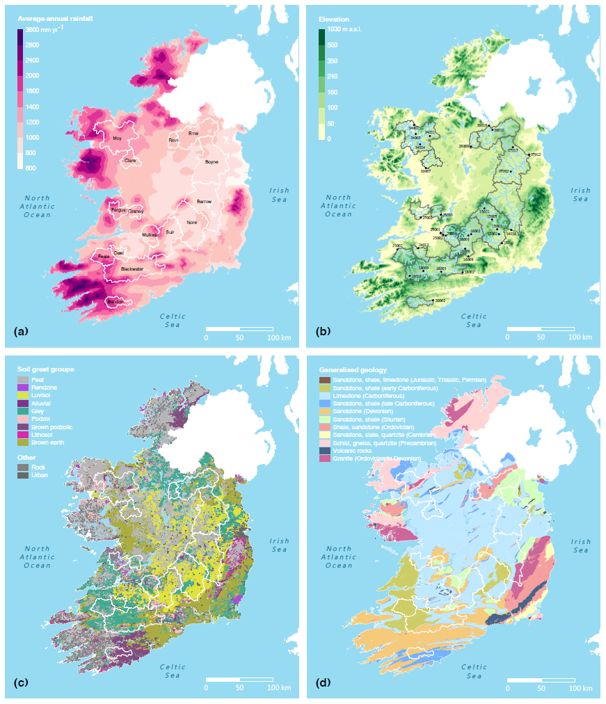
Figure 1Spatial location and information on the study catchments: (a) map of the average annual rainfall for the Republic of Ireland for the period 1981–2010 (source: Met Éireann) overlaid with the 15 distinct river basins containing the 33 study catchments – each name corresponds to a river basin; (b) map of the topography for the Republic of Ireland (source: Ireland's EPA) overlaid with the location of the 33 hydrometric gauges forming the 33 study catchments – each number corresponds to the code of a hydrometric gauge; (c) map of the pedology for the Republic of Ireland (source: Teagasc) overlaid with the outlines of the 15 river basins; (d) map of the geology for the Republic of Ireland (source: © Geological Survey Ireland) overlaid with the outlines of the 15 river basins.
Catchment selection was also influenced by the quality of the discharge data, including the goodness of fit of the rating equation at the gauge, the number of measurements, and their coverage of low-flow and high-flow extremes, as determined by Webster et al. (2017). Heavily regulated rivers were discarded. A total of 33 gauges (displayed on Fig. 1b) featured sufficient data of good quality to be used as study catchments. Of these, there are 15 distinct catchments and 18 gauges nested within these. The 15 distinct catchments (displayed on Fig. 1a) cover 26 % of the Republic of Ireland. They are spread throughout the country and represent a diversity of Irish soils and geology (Fig. 1c, d). However, while their average elevation ranges from 5 to 910 m a.s.l. (above sea level), they do not include any of the most elevated catchments in the Wicklow Mountains (relief on the eastern coast) and the mountainous edge on the Atlantic coast (Fig. 1b). Their average annual rainfall ranges from 916 to 1660 mm yr−1, and the average annual potential evapotranspiration varies from 497 to 578 mm yr−1. The size of the catchments varies from 25 to 2462 km2, and their average slope ranges from 19 to 121 m km−1. Estimated baseflow indices range from 0.31 to 0.79 (see Table A1 in the Appendix for full details).
2.3 Rainfall–runoff model
The Soil Moisture Accounting and Routing for Transport (SMART) model used here is an enhancement of the SMARG (Soil Moisture Accounting and Routing with Groundwater) lumped, conceptual rainfall–runoff model developed at National University of Ireland, Galway (Kachroo, 1992), and based on the soil layers concept (O'Connell et al., 1970; Nash and Sutcliffe, 1970). Separate soil layers were introduced to capture the decline with soil depth in the ability of plant roots to extract water for evapotranspiration. SMARG was originally developed for flow modelling and forecasting and was incorporated into the Galway Real-Time River Flow Forecasting System (GFFS) (Goswami et al., 2005). The SMART model reorganised and extended SMARG to provide a basis for water quality modelling by separating explicitly the important flow pathways in a catchment, and it has been successfully fitted to over 30 % of Irish catchments (Mockler et al., 2016).
The routing component distinguishes between five different runoff pathways: overland flow, drain flow, interflow, shallow groundwater flow, and deep groundwater flow (Fig. 2). It runs at an hourly or daily time step, requires inputs of precipitation and potential evapotranspiration, and produces estimates of discharge from the catchment. It normally has 10 parameters (Fig. 2). During energy-limited periods (i.e. when potential evapotranspiration is less than incident rainfall), the model first estimates effective or excess rainfall by applying a scaling correction θT and subtracting any direct evaporation. A threshold parameter θH determines how much (if any) of this becomes direct surface runoff through the Horton (infiltration excess) mechanism. Any surplus rainfall is assumed to infiltrate into the top layer of the soil. The soil is modelled as six layers with a total soil moisture capacity of θZ. As the moisture holding capacity of a layer is exceeded, surplus moisture moves to a deeper layer if it has capacity or else is intercepted by drains or moves to the shallow or deep groundwater stores. In water-limited periods (i.e. when potential evapotranspiration exceeds any rainfall), the model attempts to meet the evapotranspiration demand by supplying moisture from the soil layers, starting from the top layer, and incrementally moving to the lower layers, as layers become dry, with an increasing difficulty expressed by the parameter θC, until the demand is met, or all layers have dried up. Each of the above pathways is modelled as a single linear reservoir, each with its own parameter (θSK for overland and drain flow, θFK for interflow, and θGK for shallow and deep groundwater flow). The outputs of all of these are routed through a single linear reservoir representing river routing (θRK). The model does not contain any snow component, as it is infrequent in Ireland. Note that a detailed description of the conceptual model is provided in the Supplement.
Table 2List and description of the 10 parameters of the SMART model.
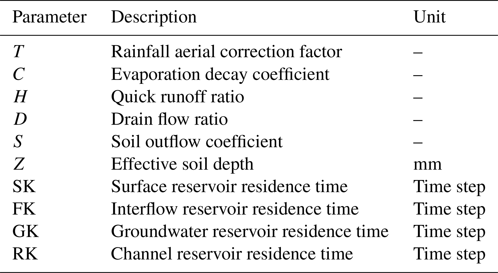

Figure 2Conceptual representation of the SMART model structure. P and EP, precipitation and potential evapotranspiration, respectively, are the model inputs; Q and EA, discharge and actual evapotranspiration, respectively, are the model outputs. For full description of the parameters, states, and fluxes presented on the figure, as well as the conceptual model equations, the reader is referred to the documentation provided in the Supplement.
3.1 Split-sample tests
Split-sample tests are commonly used to analyse the performance of hydrological models (Klemeš, 1986). Coron et al. (2012) proposed a generalised split-sample test using a sliding window of a given duration across the study period: calibration is carried out on the given window, and the model performance is evaluated for all other independent windows in the study period, thus evaluating on more than one period. This approach was simplified by de Lavenne et al. (2016) to evaluate on all data not included in the window (i.e. combining the years before and after the calibration window), thus evaluating on one period only. These approaches have the advantage of reducing any influence of different calibration–evaluation periods, compared with a single split-sample test that divides the study period into fixed, separate calibration and evaluation periods.
The split-sampling strategy in this study is adapted from the original approach by de Lavenne et al. (2016) in that it uses each hydrological year the same number of times in each of the 14 split-sample tests. For each catchment, the 14-hydrological-year series of discharge measurements is split into two 7-hydrological-year periods, and the split is repeated 14 times (Fig. 3). It is implicitly assumed that any combination of hydrological years can be used, even if they are not consecutive. Thus, there are theoretically 3432 different combinations of 7-year periods in a 14-year study period. These combinations would be expected to represent all possible climatic combinations represented in the data for the study period; however, given the large dataset this would generate, it was decided to work only on 14 combinations by using the window of 7 consecutive years, rather than more complex bootstrapping strategies.
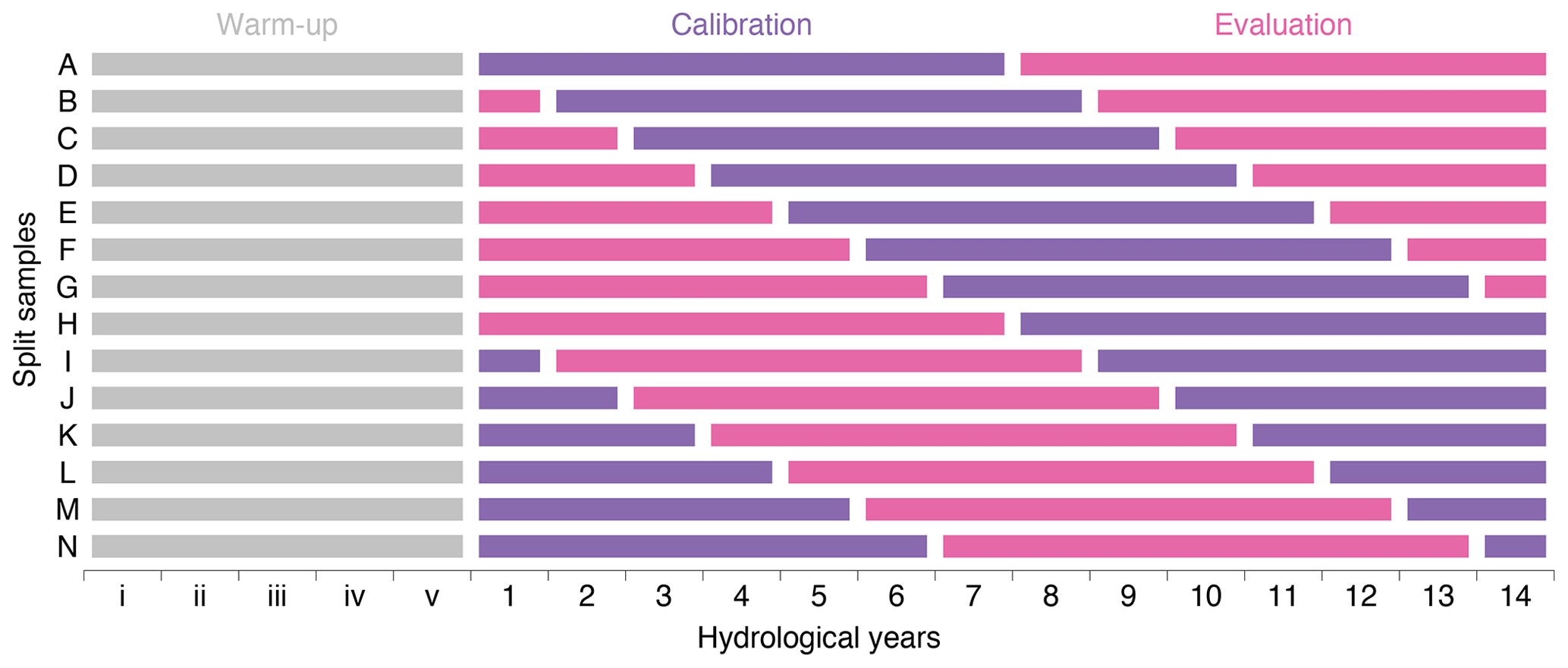
Figure 3Split-sampling strategy using a 7-year rolling window, adapted from de Lavenne et al. (2016). Each period of 14 hydrological years enumerated as decimal numerals in Fig. A1 is represented on the x axis and split into two 7-year periods, one for model calibration (in purple), and one for model evaluation (in pink). Each period of 5 hydrological years identified as roman numerals on the x axis corresponds to the 5-consecutive-year warm-up period immediately preceding the hydrological year number 1.
3.2 Model setup
The SMART model is used in a lumped manner to predict streamflow at the catchment outlet. The model is forced with daily rainfall and potential evapotranspiration data provided by the national meteorological office, Met Éireann (2019). The potential evapotranspiration is calculated by Met Éireann using the Food and Agriculture Organization of the United Nations (FAO) Penman–Monteith formula (Allen et al., 1998) with coefficients adjusted for Irish conditions and meteorological data from their synoptic weather stations. A 5-hydrological-year warm-up period is used to determine the initial states of the soil layers and reservoirs in the model. The 5-year warm-up period is applied prior to the first complete hydrological year used in the split-sample test on Fig. A1. A Python implementation of the SMART model (Hallouin et al., 2019) is used to simulate the hydrological response in all study catchments from the first day of the first warm-up year until the last day of the 14th complete hydrological year. The corresponding calibration and evaluation periods are then extracted from these time series as required (see Fig. 3).
3.3 Model calibration
The calibration of the model is done using six different objective functions. The calibration procedure is illustrated in steps (a) to (d) of Fig. 4 and is applied for each study catchment individually. First, in step (a), the model parameter space is explored using a Latin hypercube sampling (LHS) strategy (McKay et al., 1979) to generate 105 random parameter sets well distributed in the parameter space. The limits of the parameter space explored are based on a previous study by Mockler et al. (2016), providing typical ranges for Irish catchments. The model is then used in step (b) to simulate the catchment response with each of these 105 parameter sets, which produces as many hydrographs.
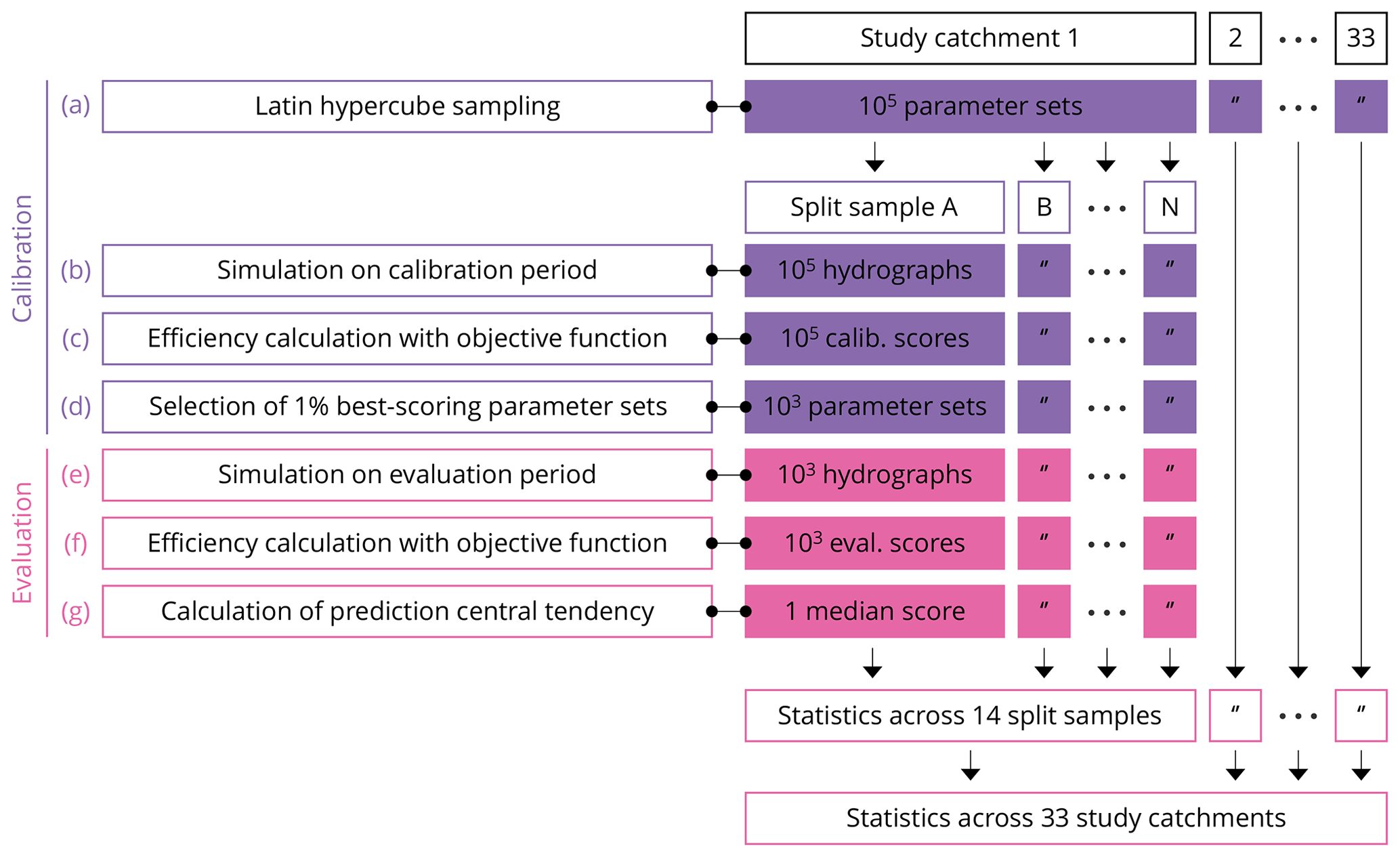
Figure 4Model calibration and evaluation strategy for the prediction of SFCs with different objective functions. Steps (a) to (d) correspond to model calibration, while steps (e) to (g) correspond to model evaluation. These steps are replicated for each study catchment and for each split-sample test.
In step (c) (Fig. 4), six different objective functions are used to calculate the model performance by comparing the simulated and observed catchment responses. Three variants of the Kling–Gupta efficiency (Gupta et al., 2009) are tested. First, the KGE criterion is computed on the untransformed discharge series, i.e. (Fig. 1). This is considered to put more emphasis on high-flow conditions (Krause et al., 2005). Second, the KGE criterion is computed on the inverted discharge series, i.e. (Fig. 2); this objective function puts more emphasis on low-flow conditions (Santos et al., 2018). Third, the KGE criterion is computed from the square root of the discharge series, i.e. (Fig. 3); this reduces the influence of high flows allowing moderate flow conditions to have a bigger influence (Garcia et al., 2017). These variants of KGE are referred to as traditional objective functions hereafter and are computed using all data points in the hydrographs. In addition, three combinations (vectors) of streamflow characteristics, referred to as tailored objective functions hereafter, are constructed. For each vector of SFCs, the Euclidean distance (Fig. 4) separating the observed and simulated points in the multi-dimensional space formed by each dimension in the vector of SFCs is calculated. This is subtracted from one so the efficiency measure has an optimum at one, like KGE. Similar to Kiesel et al. (2017), each SFC is normalised (Eqs. 5, 6) so that its value is bounded between zero and one. This ensures each SFC has the same weight in the computation of the Euclidean distance. Each of these six objectives functions are used to produce 105 efficiency scores for all the calibration cases.
Eventually, in step (d), the best 1 % parameter sets (i.e. those with the highest efficiency scores on the chosen objective function) are retained as “behavioural”, yielding a set of 103 parameter sets. This calibration approach is similar to the Generalized Likelihood Uncertainty Estimation (GLUE) methodology (Beven and Binley, 1992, 2014) but without a threshold for acceptability to characterise the behavioural character of a parameter set.
To examine the absolute performance of each of the six objective functions, a benchmark is defined by randomly sampling 103 parameter sets in the previously mentioned Latin hypercube. This benchmark corresponds to an uninformative calibration and will be referred to as R in the Results section. This follows the recommendations made by Seibert et al. (2018) to define a lower benchmark when assessing the performance of a hydrological model because any model should be expected to reproduce some of the streamflow variability simply due to the use of observed forcing data specific to the catchment of interest. If the performance of the calibrated model does not exceed the performance of the benchmark, then the suitability of the model and/or its calibration is questionable.
where cov, σ, and μ correspond to the covariance, the standard deviation, and the arithmetic mean, respectively; qobs and qsim correspond to the time series of observed discharge and simulated discharge, respectively. Noteworthy, a constant is added to the inverted discharge values in Eq. (2) in order to avoid zero-flow issues, and a hundredth of the arithmetic mean of the corresponding discharge series is used as recommended by Pushpalatha et al. (2012).
where Ntarget corresponds to the number of SFCs contained in the targeted combination of SFCs (the specific SFCs contained in each targeted combination can be found in Table 1) and where and correspond to the jth observed SFC value in the combination and the jth simulated SFC value in the combination, respectively, which were normalised as described in Eqs. (5) and (Eq. 6), respectively.
where cobs,j and correspond to the jth observed SFC value in the combination and the jth simulated SFC value in the combination for the ith streamflow simulation amongst the Latin hypercube sample, respectively.
3.4 Model evaluation
The method used to assess the predictions with a model calibrated with each of the six different objective functions is described in steps (e) to (h) of Fig. 4. This methodology is applied for each study catchment individually. First, in step (e), the model is run separately with each of the 103 behavioural model parameter sets to simulate the evaluation period, which produces 103 hydrographs. From each hydrograph, in step (f), the model prediction in the evaluation is assessed with each of the six objective functions described in Sect. 3.3, which yields 103 efficiency scores for the evaluation period. Then, in step (g), the median is used to summarise the performance of the behavioural parameter sets for each of the six objective functions in each catchment. Eventually, from these median values, further analyses are carried out across split samples and across study catchments to explore the comparative skills of the six objective functions as detailed below.
3.4.1 Overall performance
First, the overall performance for the evaluation period of the model calibrated with each of the six objective functions is assessed by averaging the median efficiency scores obtained in step (g) (Fig. 4) across the 14 split-sample tests and then averaging again across the 33 study catchments. Since all six objective functions are defined as Euclidean distances subtracted from one, the overall performance ranges from −∞ to one, with an optimal value at one. The skills of the six objective functions to calibrate the model are first compared using the traditional objective functions as efficiency scores for the evaluation period (Sect. 4.1) to assess their ability to reproduce the shape, timing, variability, and volume of the observed hydrograph. This gives an indication of whether the model structure gives a plausible approximation of the relevant hydrological processes in the study catchments.
Next, the calibrated models are compared using the tailored (SFC) objective functions for the evaluation period (Sect. 4.2) to assess their prediction of sets of streamflow characteristics. This is an important focus of this study.
3.4.2 Performance stability
The use of 14 split-sample tests allows for the comparison of the calibrated models for different evaluation periods (see Fig. 3). This gives an indication of the model stability in calibration and whether the model performance is independent of the study period. The stability is calculated from the standard deviation of the median efficiency scores across the 14 split-sample tests and is then averaged across the 33 study catchments (Sect. 4.3). This is done for all the models calibrated with each of the six objective functions. The stability can range from the optimal value of zero without an upper bound.
3.4.3 Performance robustness
The robustness of the models measures their ability to match their calibration fitting skill with their performance in the evaluation period. Poor robustness can indicate model overfitting to the calibration data, which could reduce the predictive power of the model. The robustness is calculated from the difference between the median efficiency in calibration and the median efficiency in evaluation, then by averaging these differences across the 14 split-sample tests, and finally by averaging these across the 33 study catchments (Sect. 4.4) to obtain the robustness for each of the six objective functions. The optimal value is zero, and it can be positive or negative. Robustness is expected to be positive because the performance in calibration is usually better than the performance in evaluation.
3.4.4 Consistency in the selection of the model parameter values
Finally, the model consistency obtained with each of the six objective functions is explored. The concept of consistency has been previously used in selecting from competing model structures (Euser et al., 2013). Originally used as the capacity of a model structure to predict a range of hydrological signatures with the same parameter set, in this study the idea of consistency is applied to the objective functions. The ability of different objective functions to identify the same parameter sets as behavioural is assessed across the 14 split-sample tests. Consistency establishes whether similar performance can be obtained from a model with largely different parameter sets. The consistency is computed as the fraction of the 103 behavioural parameter sets that are common to all 14 split-sample tests. The average of this fraction across the 33 study catchments is calculated (Sect. 4.5) to obtain the model consistency for a given objective function used to identify the behavioural parameter sets. The consistency ranges from zero to one, with an optimal value at one.
For this analysis, the same Latin hypercube sampling of the 105 parameter sets per catchment is used. That is to say that the Latin hypercube is generated once, and it is used on the 14 different calibration–evaluation periods in order to be able to determine whether a behavioural parameter set identified as behavioural on one test remains behavioural on a different test.
3.4.5 Analysis of the components of the objective functions
To explore the reasons for the trends identified in model performance, stability, robustness, and consistency, the ability of the six objective functions to predict the shape and timing, the variability, and the bias of the observed hydrograph is examined by assessing the three components of r, α, and β of individually from Eq. (1). Because of the transformations applied to the discharge series in and , the direct physical interpretation of their three components is lost (Santos et al., 2018), so they are not analysed further.
In addition, the ability of the six objective functions to predict each individual SFC is assessed by calculating the absolute normalised error between the simulated and the observed SFC values (Eq. 7).
where cobs,j and correspond to the jth observed SFC value in the combination and the jth simulated SFC value in the combination for the ith streamflow simulation amongst the Latin hypercube sample, respectively.
For each component analysed, the approach is the same as the one used for assessing the overall model performance in Sect. 3.4.1. This means that the median value of a given component for the behavioural parameter set is calculated; it is then averaged across the 14 split-sample tests; and it is finally averaged across the 33 study catchments to obtain an overall skill of each objective function in predicting these individual components.
3.4.6 Analysis of the performance on a large set of SFCs
Finally, the comparative performance of the objective functions to calibrate the hydrological model is assessed on 156 different SFCs and the 9 percentiles of the flow duration curve where Eq. (7) is used to determine the predictive errors. This analysis is intended to provide a more holistic picture of the skills of the different objective functions in predicting different flow conditions (i.e. low, moderate, and high flows) and different flow characteristics (i.e. magnitude, duration, frequency, timing, and rate of change).
4.1 Are the candidate objective functions capable of reproducing the catchment hydrograph?
The SMART model calibrated on does reproduce the observed catchment hydrographs reasonably well in all 33 study catchments, with average scores in calibration across the 14 split-sample tests ranging from 0.58 to 0.94 with a median of 0.86.
On average, all six objective functions reproduce the observed hydrograph well when more weight is given to predicting high flows, with scores in the evaluation between 0.69 and 0.82 (Fig. 5a). They largely outperform the average benchmark score of 0.40, indicating that all six objective functions do find parameter sets representative of the hydrological behaviour of our catchments. Using for calibration is the best objective function when measured using with a score of 0.82, followed by with a score of 0.80. However, is outperformed by the three tailored objective functions. is the best tailored objective function when measured on , followed by and . This is because and contain a majority of SFCs for high-flow conditions (Table 1), while contains a majority of SFCs for low-flow conditions.
When more importance is given to predicting average-flow conditions, i.e. using (Fig. 5b), the best-performing objective function is with a value of 0.87,, followed by with 0.86 and the three tailored objective functions with very comparable performances (between 0.84 and 0.85). Since the three tailored objective functions contain comparable proportions of SFCs for average-flow conditions (i.e. around 30 %, see Table 1), it can explain why their values of are close.
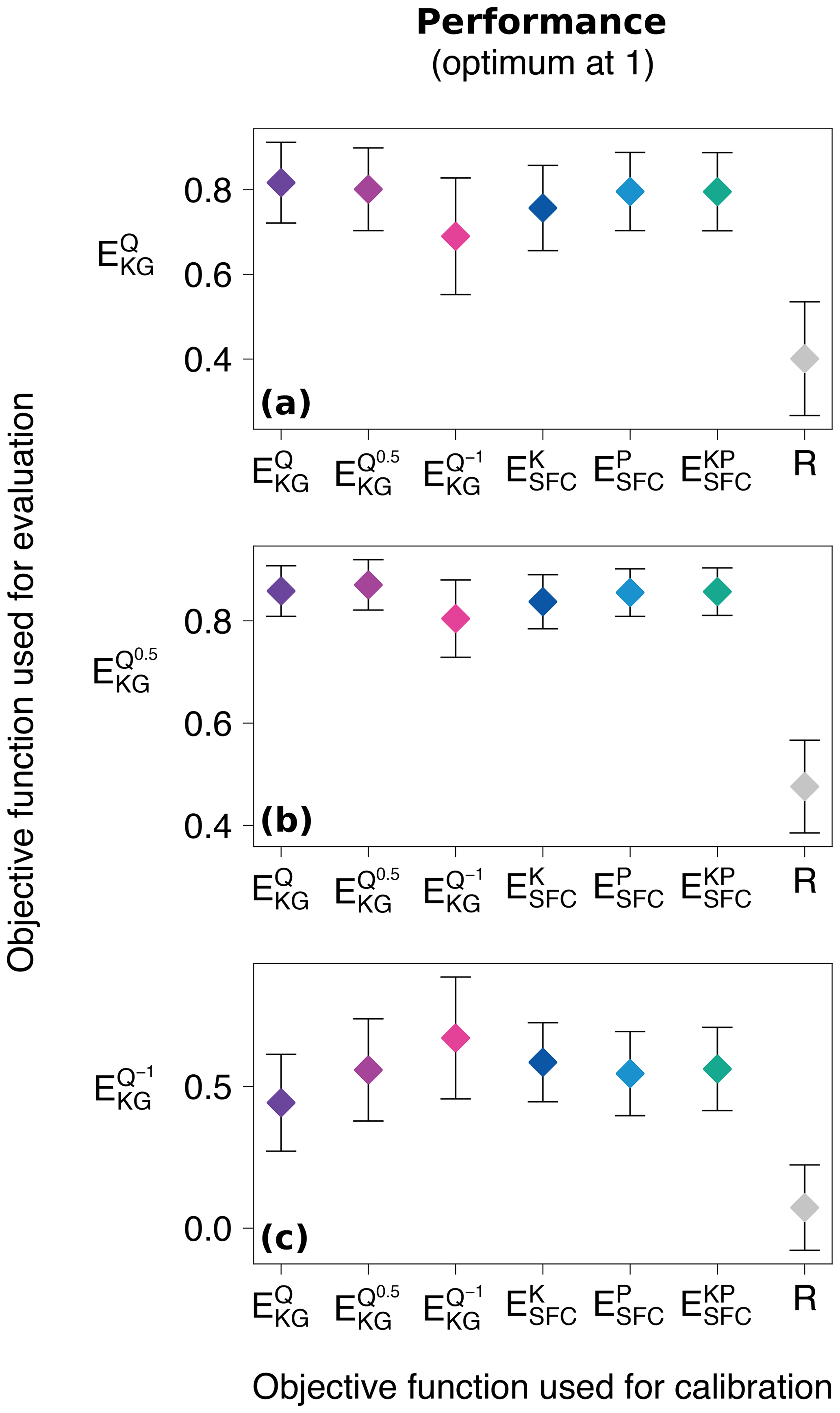
Figure 5Comparison of the overall performance in evaluation of the model calibrated with the six objective functions. The three traditional objective functions are used as evaluation efficiencies. corresponds to the original Kling–Gupta efficiency (Gupta et al., 2009).
While is the worst objective function when assessed on or , when more emphasis is put on low flows, i.e. assessed using (Fig. 5c), it performs the best out of the six objective functions with a score of 0.67, followed by with a score of 0.59. and perform equally with a score of 0.56, while has a score of 0.55. is the worst objective function to choose out of the six to predict low flows well. Nonetheless, it is better than the lower benchmark with its score of 0.07. Again, the proportion of low-flow SFCs explains the ranking of the three tailored objective functions, where features three SFCs for low-flow conditions out of its seven SFCs (see Table 1), while features the lowest proportion of SFCs for low-flow conditions (i.e. 4 out of 13; Table 1).
4.2 Which objective function provides the most accurate SFC predictions?
The differences between most of the objective functions are small (Fig. 6a–c). They greatly exceed the benchmark on all three tailored objective functions, indicating that all six objective functions are useful. The best evaluation scores for a given set of SFCs is always obtained using the same combination of SFCs in evaluation as was used in calibration; e.g. the best score in evaluation (0.74) is obtained with as the objective function for calibration. ( scores 0.56 on ; scores 0.50 on .) Furthermore, for the combination with the largest number (18) of SFCs, is a competitive option, even when the focus is on smaller subsets of SFCs (i.e. scores 0.73 on or scores 0.56 on ), and it outperforms any of the three formulations of EKG.
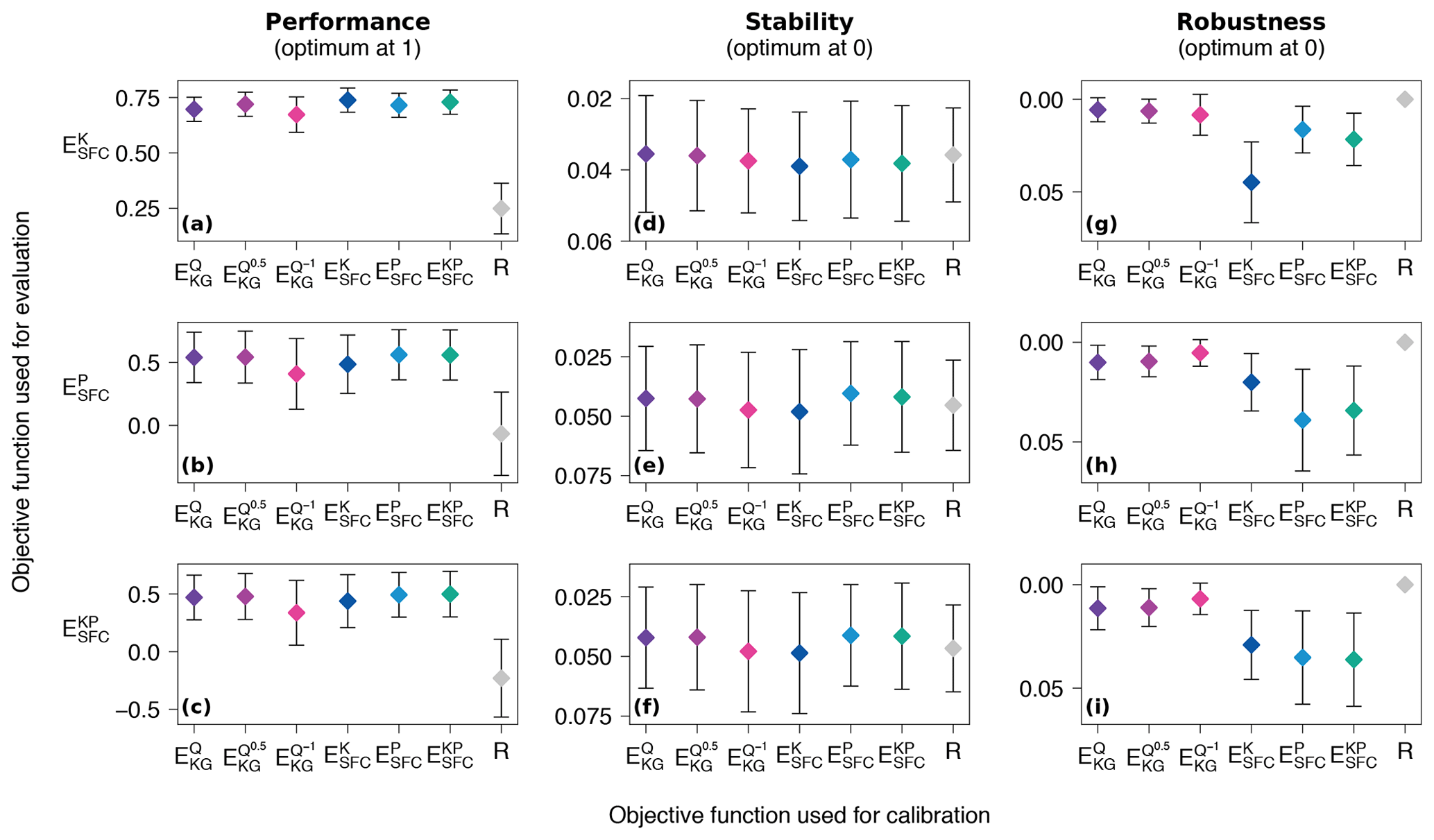
Figure 6Comparison of the skills in evaluation of the model calibrated with the six objective functions. The first column of panels compares them on the overall performance on the three tailored objective functions used as evaluation efficiencies (described in Sect. 3.4.1). The second column compares them on the stability of these efficiencies across the 14 split-sample tests (described in Sect. 3.4.2). The third column compares them on the robustness of these efficiencies between calibration and evaluation periods (described in Sect. 3.4.3).
The best traditional objective function to predict any of the sets of SFCs is consistently , with scores of 0.72 on , 0.54 on , and 0.48 on . is the worst-performing traditional objective function, with scores of 0.67 on , 0.41 on and 0.34 on . Given that contains the highest fraction of low-flow SFCs (three out of seven), it is surprising to find the traditional objective function with the strongest focus on predicting low-flow conditions is the worst-performing one. However, Garcia et al. (2017) also found that is not the best to predict low-flow indices and recommend an arithmetic mean of and as a better alternative to predict them.
In addition, the dispersion of the performance across the 33 study catchments, measured by standard deviation (represented as error bars on Fig. 6a–c), is smaller for the better-performing objective functions, which indicates that in addition to predicting well on average, they have less variability across the different study catchments.
4.3 Which objective function provides the most stable SFC predictions?
The average stability of the performance across the 14 split-sample tests shows only small differences between the different objective functions (Fig. 6d–f). Moreover, the absolute stability scores, measured by the standard deviation across the 14 split samples (see Sect. 3.4.2), are also relatively small, i.e. never exceeding 0.05. Here, the benchmark is as stable as the six objective functions used for calibration. This suggests that stability is not very useful here to separate the objective functions given that an uninformative calibration yields similar stability. Their small values imply that the differences observed previously are not dependent on the study period considered.
4.4 Which objective function provides the most robust SFC predictions?
The robustness of the different objective functions on the three sets of SFCs uncovers a general trend whereby traditional objective functions are more robust than tailored objective functions; i.e. the drop in performance from the calibration period to the evaluation period is smaller for the traditional objective functions (Fig. 6g–i).
The average drop in performance is consistently below 0.01 for , , and on all three sets of SFCs. On the other hand, the largest drop in performance on any of the three sets of SFCs is always obtained with this same set used in calibration. For instance, shows an average drop of 0.045 on , while the drop is only 0.016 with and 0.022 with . This difference in robustness may be caused by tailored objective functions suffering more from overfitting than the traditional objective functions. Nonetheless, the tailored objective functions remain the best options when considering results in the evaluation period so that although they reach better fitting in calibration, it is at the cost of larger performance drops from calibration to evaluation. These results are consistent with Garcia et al. (2017), who also found that their tailored objective function made of seven SFCs was not robust.
4.5 Which objective function yields the most consistent behavioural parameter sets?
Unlike the measures of average model performance and stability, the consistency measures reveal more significant differences between the six objective functions compared here (Fig. 7). On average, and clearly outperform all other objective functions with consistencies of 0.52 and 0.51, respectively. This means that more than half of the behavioural parameter sets identified with these two objective functions remain behavioural across all 14 split-sample tests. The lowest consistencies are for and with 0.19 and 0.13, respectively. These focus mostly on low-flow conditions, and this may contribute to their lack of consistency.
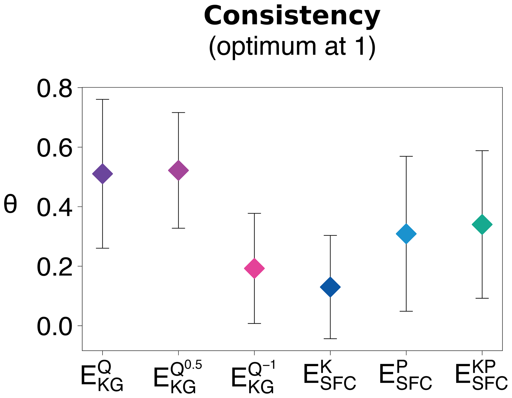
Figure 7Comparison of the consistency of the set of behavioural parameter sets identified with the six objective functions across the 14 split-sample tests (described in Sect. 3.4.4).
The consistency ratios for the tailored objective functions appear to be related to the number of SFCs they contain. For instance, , containing only seven SFCs, comes last with a consistency of 0.13; with 13 SFCs has a consistency of 0.31; and , containing all 18 SFCs, has a consistency of 0.34. However, given that only three sets of SFCs are tested, this could be a coincidence, and additional research on the impact of the number of SFC components in the tailored objective functions on their consistencies is indicated.
4.6 Are there specific components of the objective functions limiting their performances?
4.6.1 Shape and timing, variability, and bias
First, comparing the six objective functions on the three components of (Fig. 8) reveals that the shape and timing (r) is the most difficult aspect of the hydrograph to predict, while the total volume (β) is the least difficult. The flow variability (α) is consistently underestimated, while the total volume is overestimated with all but one objective function (i.e. ).
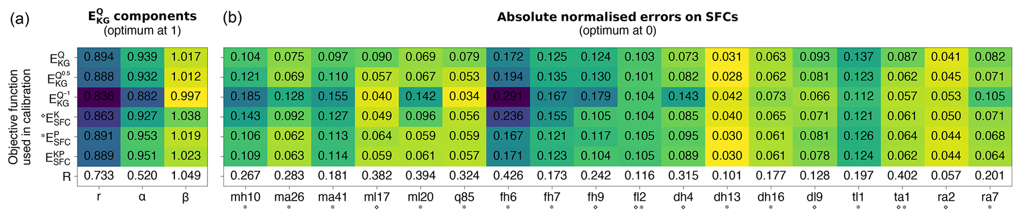
Figure 8Comparison of performance in evaluation of the model calibrated with the six objective functions on individual components of the objective functions. Panel (a) compares them on the three components of the Kling–Gupta efficiency. Panel (b) compares them on the individual SFCs that are contained in the three tailored objective functions. A hollow diamond and an asterisk are used to display the SFCs belonging to and to , respectively. Note that all SFCs belong to .
performs the worst on two of the three components, with a score of 0.836 on the linear correlation r and 0.882 on the variability α. This indicates that the objective function struggles the most to reproduce the shape and timing of the observed hydrograph, and also it is the one that most underestimates the observed spread of flows. On the other hand, it is the best objective function to estimate the volume of water at the catchment outlet (score of 0.997 on β). On the other hand, and perform well on α and β, while they are not as good on the correlation coefficient r. Nevertheless, they are better than most other objective functions on r, with amongst the highest scores on r (0.894 and 0.888, respectively).
The bad performance of found in Sect. 4.1 can be attributed mainly to a lower correlation component of , with a value of 0.863, and to a lesser extent to a failure to capture the flow variability (α value of 0.927). Even though is the worst objective function for bias (β has a value of 1.038), this is its best score amongst the three components of . and are good at capturing the flow variability, with α values close to one (0.953 and 0.951, respectively). They are comparable to and on the correlation coefficient, while they overestimate the total volume the most (1.018 and 1.022 for the bias, respectively).
and share an emphasis on low-flow periods that is likely the reason compromising their performance on the linear correlation coefficient r, which gives more weight to high-flow periods. High-flow periods typically exhibit larger errors that are amplified by the quadratic formulation of the correlation coefficient (Krause et al., 2005). Moreover, and contain higher proportions (and larger numbers) of SFCs relating to flow magnitude than (Table 1), which can explain why is worst on the bias component. Finally, and contain two SFCs for the timing of flows, while contains only one, which can explain why is not as good as the two others for the correlation coefficient.
4.6.2 Individual streamflow characteristics
The normalised errors for the 18 SFCs that are contained in the three tailored objective functions (Fig. 8) show that, overall, all six objective functions tend to produce the largest errors for the same SFCs, for example on fh7 (frequency of large floods), fh6 (frequency of moderate floods), or tl1 (timing of annual minimum flow). Also the smallest errors are produced for the same SFCs, for example dh13 (variability in annual minimum 30 d mean flow) or ra2 (variability in flow rise rate). The prediction of the SFCs considering the frequency of flow events (fh6, fh7, fh9, and fl2) is the most difficult with all six objective functions, while SFCs related to their duration (dh4, dh13, dh16, and dl9) are amongst the easiest to predict. For the magnitude of flow events, low-flow events seem to be relatively easy to predict compared to the magnitude of average- and high-flow events.
However, and tend to show more variability than the other four objective functions in the ranking of the errors across the 18 SFCs. For example, shows larger errors on SFCs related to high-flow conditions (mh10, fh6, fh7, fh9, and dh4) because of the focus on low flows of the objective function but also on some average-flow conditions (ma26, ma41, and ra7) and even on low-flow SFCs (ml20 – baseflow ratio). This is also the case for mostly the same SFCs with . Again, these two objective functions place more emphasis on low flows, and this seems to make them less suitable across a wider range of flow conditions. On the other hand, the emphasis on high flows in seems less detrimental to its performance on low-flow conditions. Although it is worst of all on ml17 (baseflow ratio) and q85 (flow exceeded 85 % of the time), it is still with relative errors below 10 %.
Unlike the overall performance behaviour described in Sect. 3.4.1, a tailored objective function does not necessarily perform the best on all of the individual SFCs it contains. For example, outperforms on ma41 (annual mean daily flow), which was already noticed with the bias. Also, outperforms on q85, which can be explained by the strong emphasis puts on low flows. Interestingly, a tailored objective function can outperform another one on SFCs it does not contain. Indeed, outperforms on ra2, even though the latter is only contained in .
4.7 Trends on a large range of flow regime characteristics
Extending the number of SFCs examined shows that , , and perform very similarly across the 156 SFCs and the 9 percentiles of the flow duration curve (Fig. 9) and that they are somewhat similar to , except for the magnitude and duration of low-flow events, where produces larger errors. This implies that is a good choice for model calibration when the purpose is to predict a wide range of streamflow characteristics across various flow conditions, since it performs almost as well as the best tailored objective functions. In contrast, produces noticeably larger errors than any other objective function on the maximum daily flow in each month (i.e. mh1 to mh12), on the mean annual maximum of a moving mean of a 1, 3, 7, 30, and 90 d window (dh1 to dh5), or on the frequency of flood events of various intensities (fh1, fh5, fh6, and fh8). At the same time, this objective function produces markedly smaller errors on the mean annual minimum of a moving mean of a 1, 3, 7, 30, and 90 d window (dl1 to dl5). Overall, the stronger weight on low-flow conditions of does improve the predictions of SFCs for low-flow events to the detriment of the prediction for high-flow events. This is also noticeable in the percentiles of the flow duration curve, with an almost monotonic increase in the error amplitude from the 99th percentile to the 1st percentile. However, is the worst objective function for predicting the minimum daily flow in each month for the period October–February (ml10, ml11, mh12, ml1, and ml2). This is because the magnitude of low flows during this wet period are higher than during the dry period so that errors for low flows for the dry period are given a higher weight than the ones for the wet period in . Also, it has a larger error for predicting the frequency of low-flow periods (fl1); this is because the threshold for low-flow periods is set as the 25th percentile, which is not the magnitude of flows that is the most emphasised by (i.e. not on the lower tail of the flow distribution).
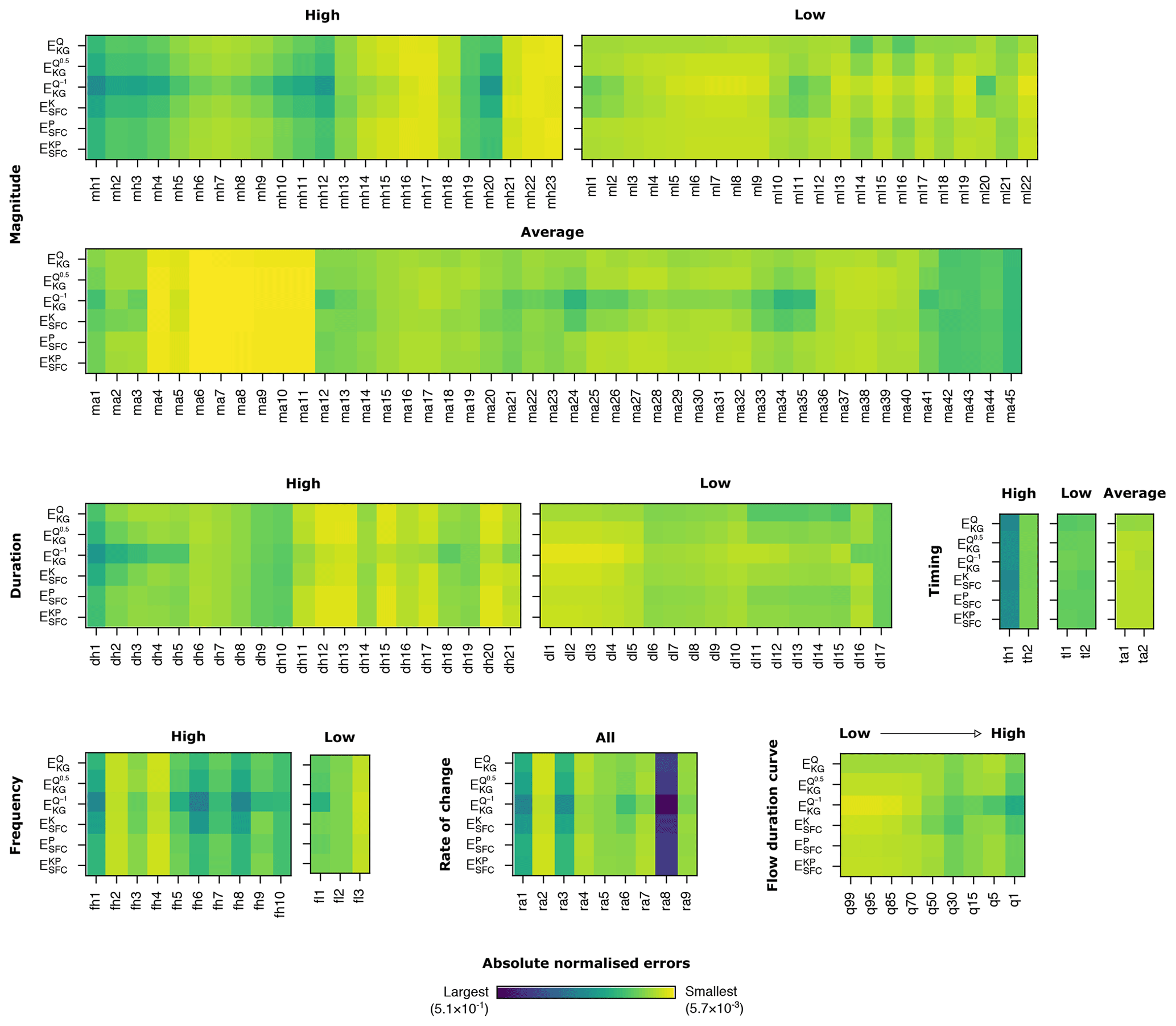
Figure 9Comparison of performance in evaluation of the model calibrated with the six objective functions on 156 streamflow characteristics and 9 percentiles of the flow duration curve. A detailed description of each SFC can be found in the Appendix of Olden and Poff (2003).
Amongst the tailored objective functions, performs differently across the 156 SFCs and the 9 percentiles than its two counterparts, which perform very similarly across these SFCs. Indeed, shows absolute normalised errors between and the two other tailored objective functions. tends to show larger errors on the characteristics where is outperformed by the other traditional objective functions, typically on characteristics for low-flow conditions. This pattern was already observed on the smaller set of SFCs in Sect. 4.6.2.
Beyond the patterns identified above, the relative agreement in the SFCs showing the largest and smallest errors across the six objective functions provides some insight on the easiest and hardest SFCs to predict. It is clear that the average number of flow reversals from one day to the next (ra8) is the most difficult to predict and so are, to a lesser extent, the average slope of the rising and recession limbs (ra1 and ra3). Overall, high-flow events are trickier to predict, whether it is their magnitude (mh1–mh12 – mean daily maximum for each month, mh19 – skewness in annual maximum daily flow, and mh20 – mean annual maximum daily flow), their duration (dh1–dh10 – mean and variability in annual maximum of a moving mean of a 1, 3, 7, 30, and 90 d window), their timing (th1 – timing of annual maximum flow), or their frequency, except for the variability in high-flood events (fh2) and the average number of days exceeding 7 times the median flow (fh4). On the other hand, some SFCs based on the magnitude of flows are easier to predict, e.g. variability in the percentiles of the log-transformed discharge record (ma4), the skewness in daily flows (ma5), various ratios of flow percentiles (ma6-ma8), and various spreads between flow percentiles (m9–m11). The volume of floods exceeding the median, twice the median, and 3 times the median (mh21, mh22, and mh23) are also well predicted, alongside the 90th and 75th percentiles normalised by the median flow (mh16 and mh17). Finally, the mean annual maximum of a moving mean of a 7 and 30 d window normalised by the median flow (dh12 and dh13) are the best-predicted SFCs relating to the duration of flows. For the percentiles of the flow duration curve, it appears that all six objective functions are better suited to predicting its low tail, which is consistent with the lower relative errors for the SFCs on the magnitude of low flows compared with those of high flows.
5.1 On the definition of SFC-based objective functions for ecologically relevant streamflow predictions
The choice of the objective function for ecological applications influences the predictive performance of the hydrological model for specific streamflow characteristics (Vis et al., 2015; Kiesel et al., 2017; Pool et al., 2017). In particular, specially chosen composite objective functions containing the target SFCs have improved the prediction of these SFCs (e.g. Kiesel et al., 2017). This study confirmed these separate findings using the same set of SFCs in Irish study catchments. However, the consistency analysis done here reveals that the parameter sets identified in the calibration are less consistent across different split-sample tests with this type of objective function than with two of the traditional objective functions (i.e. and ).
The selection of particular streamflow characteristics for their ecological relevance does not imply that they can represent the overall hydrograph. Indeed, while some indicators originally used as ecologically relevant SFCs (Olden and Poff, 2003) are also used as hydrological signatures (e.g. Yadav et al., 2007; Zhang et al., 2008), their selection as a relevant characteristic for a catchment is driven by the requirement to model specific indicators. These indicators can be ecologically relevant SFCs according to their influence on the stream ecology (Poff and Zimmerman, 2010), while they are also selected as hydrological signatures to represent the hydrological behaviour of catchments (McMillan et al., 2017). In such cases, they are SFCs that can be used for catchment classification or the regionalisation of hydrological information, for example. Ecologically relevant SFCs are not necessarily very informative when it comes to estimating suitable parameter values in the calibration of hydrological models, because they may not be key descriptors of the key hydrological processes at the catchment scale. This may be symptomatic of the problem of getting the right answer with a model for the wrong reasons (Kirchner, 2006). For example, Pool et al. (2017) defined a composite objective function made of the most informative SFCs at hand (i.e. the ones that, used alone, were the most useful to predict the other SFCs well too), and yet, they were unable to accurately predict SFCs not included in the objective function. The use of a consistency analysis in this study confirms that the tailored objective functions tested are not skilled in selecting parameter values stable across split-sample tests. Nonetheless, some SFCs are useful in calibration. Yadav et al. (2007) suggest that a carefully selected subset of SFCs has the potential to constrain a model parameter space. Kiesel et al. (2017) even found that the use of single SFCs may be almost as powerful as their complete set of seven SFCs to predict all seven SFCs, suggesting that some ecologically relevant SFCs also have potential to be indicative signatures of the hydrograph of their German catchment.
In this context, the definition of a good tailored objective function for ecologically relevant streamflow predictions must be based on SFCs that are key descriptors of the ecological response while also being key descriptors of the hydrological behaviour in the catchment. Otherwise, model consistency may be compromised, and the model predictions will not be as robust outside its calibration conditions. Moreover, the number of SFCs contained in the tailored objective function needs to be considered, given that consistency seems to improve with the number of SFCs contained in the objective function. However, as only three different sets of SFCs were tested in this study, more research would be required to confirm this hypothesis.
5.2 On the strengths of traditional objective functions
Composite traditional objective functions such as the Kling–Gupta efficiency are strong contenders for the prediction of these SFCs. In particular, the use of the KGE on square-rooted flows (i.e. ) was as competitive as tailored objective functions while providing more robust predictions and a more consistent set of behavioural parameter sets than its tailored counterparts. On the other hand, the stronger focus on low-flow errors of reduces its ability to predict SFCs for high-flow events, which is a disadvantage, unless the ecological species of interest are only sensitive to low-flow conditions. Even then, Garcia et al. (2017) found an arithmetic mean of and was better than alone to predict low-flow SFCs. Conversely, the heavier emphasis on high-flow errors of is not as detrimental for its prediction of low-flow events and is only marginally worse than .
In future research on the skills of objective functions to predict SFCs, a recently formulated non-parametric version of the KGE criterion could prove useful to predict various SFCs at once. It reduces the emphasis on high-flow conditions, and it provides a more balanced criterion across various flow conditions while avoiding the assumptions on the nature of the errors of the original KGE not necessarily justified for streamflow records (Pool et al., 2018). Alternatively, segments of the flow duration curve have been used to calibrate hydrological models, which also offers opportunities to balance low-, average-, and high-flow conditions (e.g. Yilmaz et al., 2008; Pfannerstill et al., 2014). However, the flow duration curve does not contain information on the timing (or duration) of individual flow events, which is important for aquatic species (Arthington et al., 2006). A combination of different objective functions fitted to flows (Vis et al., 2015) or a combination of objective functions fitted to flows and objective functions fitted to SFCs (Pool et al., 2017) can also be competitive options. In particular, the latter has the potential to overcome the consistency issue found with tailored objective functions by including traditional objective functions.
5.3 Limitations of this study
The lack of long continuous time series of observed streamflow is known to be a limiting factor for ecohydrological studies, and, in this case study, the use of 14 years, i.e. 7 years each for the calibration and evaluation periods, is a prime example of this issue. Previous research suggests that a 5-year period is enough to capture the temporal hydrological variability (Merz et al., 2009). However, Kennard et al. (2009) found that at least a 15-year period was required to accurately estimate a set of 120 SFCs, where the true SFC values were taken from their full record of 75 years. This suggests that the SFC values targeted in calibration in this study may not be fully representative of the long-term hydrological regime, and they are likely to be more variable and more difficult to predict than long-term values. Indeed, Vigiak et al. (2018) found that the uncertainty in the prediction of SFCs is sensitive to the length of the period considered. Moreover, shorter time series reduce the likelihood of encompassing the most extreme flow events (droughts and floods).
In order to overcome the lack of long time series of streamflow data, we included non-continuous (i.e. interrupted) data periods to increase the number of study catchments (see Fig. A1). Given that missing discharge data tend to be more frequent for high flows because of flood events damaging the gauge, there is a risk that the natural flow variability is underestimated; and as a consequence the observed SFC values for extreme flow conditions may be less representative than other SFC values. In our study, some hydrological years were discarded even if 1 d of observations was missing. In future research, this requirement could be relaxed and infilling methods could be used on gaps of a short length to infer the values for the missing days in the streamflow series (see e.g. Gao et al., 2018, for a recent review of such imputation methods).
Given forcing and evaluation data uncertainty and model structural uncertainties, the small differences in model performance calibrated with the different objective functions could be considered insignificant. However, to reduce the influence of data uncertainty, this comparison of objective functions was carried out on a set of 33 study catchments and on 14 split-sample tests. Moreover, the use of the median performance across a set of behavioural parameter sets reduces the influence of equifinality problems (Beven and Freer, 2001). Given that summary statistics across the split-sample tests and across the study catchments are used, this may explain why differences in performance are small. Regardless, the differences in terms of model robustness and consistency are more significant and give some confidence in the general applicability of these findings.
The findings in this study could also be somewhat model specific and region specific. However, Caldwell et al. (2015) found that the choice of the hydrological model to predict SFCs is not as important as the choices of the calibration strategy, and this study confirms the results of two other similar studies (Kiesel et al., 2017; Pool et al., 2017) that tailored objective functions perform better than traditional ones. In addition, the model suitability for the study catchments could be further explored following the covariance approach recently suggested by Visser-Quinn et al. (2019), and this could potentially improve on the model consistency.
Finally, the analysis of the consistency was based on the number of times the exact same parameter set was identified as behavioural across the 14 split-sample tests. However, it is possible that in some split-sample tests, a parameter set identified as behavioural is near another parameter set also identified as behavioural in another test. This is one limitation of the consistency approach selected here, and it is suggested that future research efforts on the topic could use clustering analysis techniques in order to overcome this limitation by comparing the spread of the cluster(s) formed by the behavioural parameter sets instead.
5.4 Implications for the study of the impacts of climate change on the stream ecology
Hydrological models are usually preferred over statistical regression models when the impacts of a changing climate on the flow regime and the associated ecologically relevant SFCs is of interest. Even though regression models may fit historical calibration data better (Murphy et al., 2013), hydrological models have better potential to be run with alternative climate data in order to predict future changes in the catchment hydrograph. The identification of the most suitable objective function is therefore valuable for climate change scenario analysis. Here, we have established the marginal superiority of tailored objective functions over a range of 14th different split-sample tests in which the ranking between the objective functions is relatively stable. However, a limitation of the study is that the flow data period from 1986 to 2016 is relatively short in climatological terms and does not contain a drought period as severe, as some have been identified from long-term (250-year) precipitation records (Noone et al., 2017), since a corresponding flow record does not exist.
Assuming a suitable set of SFCs has been found, as described in Sect. 5.1, the use of a composite definition for the objective function based on normalised absolute error between observed and simulated SFCs may not be realistic for practical applications. Indeed, while SFCs are often normalised to avoid artificially weighing them based on their amplitude, they are not weighed according to the impact a given percentage deviation has on the stream ecology. The use of an objective function whose components are weighted according to their significance to the target species may therefore prove useful to include. For example, Visser-Quinn et al. (2019) used variable limits of acceptability for the identification of the plausible model parameter sets based on a weighing scheme considering the importance of each of their SFCs on the ecological response, using macro-invertebrates as a surrogate (Visser et al., 2018).
5.5 Implications for ecologically relevant streamflow predictions in ungauged basins
Understanding the ecological response to altered flow regimes is hindered by the lack of corresponding hydrological data (Poff et al., 2010) because hydrometric gauges may not be in the same locations as ecological surveys. As a result, the usual data-based calibration of a hydrological model for the ecological survey sites is not possible, and an indirect method of predicting streamflow characteristics in ungauged locations is required.
One approach to regionalisation is the transfer of optimised parameter values from gauged to ungauged locations (Parajka et al., 2005). Given their higher consistency demonstrated in this study, the original KGE-based criteria appear better suited for regionalisation than the tailored objective functions tested in this study. Indeed, the optimised parameter values need to be strongly related to catchment behaviour and physical features to be transferable to ungauged locations. While consistency could be improved through a change in model structure (Euser et al., 2013), Caldwell et al. (2015) and Garcia et al. (2017) found the choice of the calibration procedure more decisive than the model used for the prediction of SFCs.
Alternatively, streamflow characteristics can be directly transferred from gauged to ungauged locations (e.g. Yadav et al., 2007; Westerberg et al., 2014) and used as calibration information in the ungauged catchment. However, these SFCs are used as hydrological signatures to constrain the model parameter space, and as a result, their potential was assessed in order to predict the hydrograph in ungauged catchments. It remains to be explored whether these regionalised ensemble predictions can prove useful in predicting other SFCs relevant for ecological communities in ungauged catchments.
Desirable qualities for a useful objective function are that it identifies model parameter values that perform well in the evaluation, i.e. outside calibration and independent of the period considered, and that it consistently identifies the same parameter sets regardless of the study period, i.e. that it describes a consistent catchment hydrological behaviour. This study explored these aspects for six different objective functions intended to predict three combinations of streamflow characteristics that are assumed to be relevant for stream ecology. In relation to the research questions presented in the Introduction, the study showed that tailored objective functions (fitted to SFCs) perform marginally better than traditional objective functions (fitted to flows) in predicting all three combinations of SFCs on average (Q1), while proving to be less robust outside calibration than their traditional counterpart (Q2); no general trend could be found to support the claim that any objective function yields more stable SFC predictions across the split-sample tests (Q3); and traditional objectives functions fitted to untransformed flows and to square-rooted flows select more consistently the same parameter sets as behavioural across the split-sample tests than any of the three tailored objective functions made of SFCs (Q4). In addition, it was found that the ranking of the six objective functions is not altered when considering their performance on a very large and diverse set of SFCs.
This study reveals that a gain in fitting performance for the SFCs may be at the expense of consistency in the behavioural parameter sets across the split-sample tests. This highlights that fitting ecologically relevant SFCs well is not necessarily a guarantee of representing all the key hydrological processes (i.e. informative signature) defining the catchment response. Unless streamflow characteristics are proven to be both ecologically relevant and an informative signature at once, carefully selected traditional objective functions fitted to flows are likely to remain preferable to predict ecologically relevant streamflow predictions to avoid consistency issues.
Table A1List and main characteristics of the 33 study catchments.
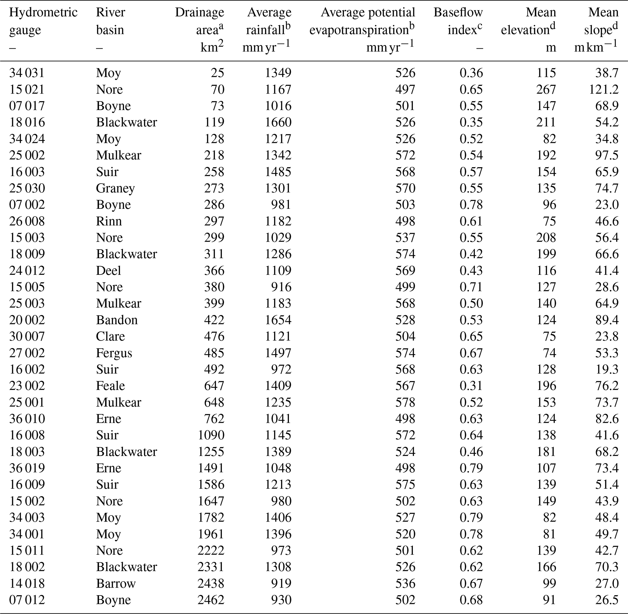
Data sources are the a EPA river sub-basins map; b Met Éireann weather stations; c Office of Public Works Flood Studies Update; and d EPA digital terrain model.
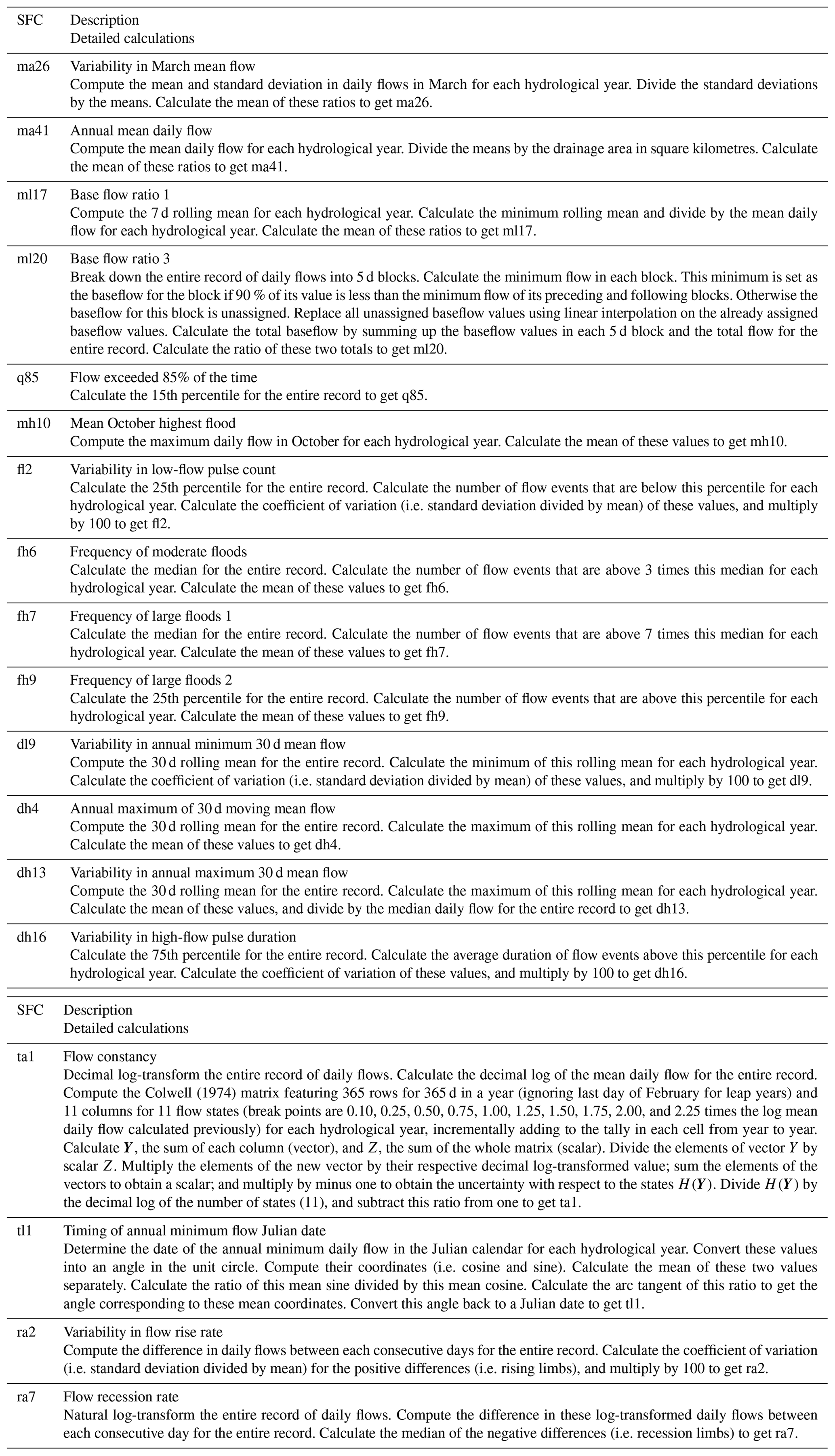
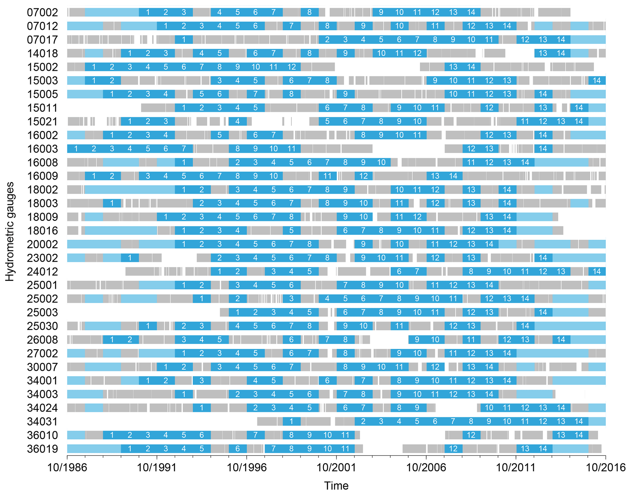
Figure A1Discharge data availability for the 33 study catchments. The 14 complete hydrological years selected are represented in dark blue and annotated from 1 to 14. Years in light blue are other complete hydrological years that are not retained. Grey years with missing data are represented as bars with discontinuities.
The rainfall and potential evapotranspiration daily datasets are available online from Met Éireann (2019). The streamflow observations are available online from Ireland's Environmental Protection Agency (2019) and from the Office of Public Works (2019). The source code of the SMART model is open source and accessible online (Hallouin et al., 2019) (https://doi.org/10.5281/zenodo.2564042). The source code for the tools used to calculate the streamflow characteristics and the traditional objective functions are also open source and accessible online (Hallouin, 2019a, b) (https://doi.org/10.5281/zenodo.2591218).
The supplement related to this article is available online at: https://doi.org/10.5194/hess-24-1031-2020-supplement.
This work is part of the PhD research of TH at the UCD Dooge Centre for Water Resources Research under the supervision of MB and FEO'L. TH developed the idea. TH collected the data and performed the model simulations. TH wrote the original draft, edited the different drafts, and produced the final version of this paper. MB and FEO'L reviewed and edited the different drafts and the final version of this paper.
The authors declare that they have no conflict of interest.
The authors would like to thank the editor and the anonymous reviewers for their comments and suggestions that contributed to improving this paper.
This research has been supported by the Ireland's Environmental Protection Agency (grant no. 2014-W-LS-5).
This paper was edited by Jan Seibert and reviewed by Cristina Prieto and two anonymous referees.
Allen, R. G., Pereira, L. S., Raes, D., and Smith, M.: FAO Irrigation and Drainage Paper No. 56, Crop Evapotranspiration: Guidelines for computing crop requirements, Tech. rep., FAO, Rome, Italy, 1998. a
Archfield, S. A., Kennen, J. G., Carlisle, D. M., and Wolock, D. M.: An Objective and Parsimonious Approach for Classifying Natural Flow Regimes at a Continental Scale, River Res. Appl., 30, 1166–1183, https://doi.org/10.1002/rra.2710, 2014. a, b
Arthington, A. H., Bunn, S. E., Poff, N. L., and Naiman, R. J.: The challenge of providing environmental flow rules to sustain river ecosystems, Ecol. Appl., 16, 1311–1318, https://doi.org/10.1890/1051-0761(2006)016[1311:TCOPEF]2.0.CO;2, 2006. a, b
Beven, K.: A manifesto for the equifinality thesis, J. Hydrol., 320, 18–36, https://doi.org/10.1016/J.JHYDROL.2005.07.007, 2006. a
Beven, K.: Facets of uncertainty: epistemic uncertainty, non-stationarity, likelihood, hypothesis testing, and communication, Hydrolog. Sci. J., 61, 1652–1665, https://doi.org/10.1080/02626667.2015.1031761, 2016. a
Beven, K. and Binley, A.: The future of distributed models: Model calibration and uncertainty prediction, Hydrol. Process., 6, 279–298, https://doi.org/10.1002/HYP.3360060305, 1992. a
Beven, K. and Binley, A.: GLUE: 20 years on, Hydrol. Process., 28, 5897–5918, https://doi.org/10.1002/hyp.10082, 2014. a
Beven, K. and Freer, J.: Equifinality, data assimilation, and uncertainty estimation in mechanistic modelling of complex environmental systems using the GLUE methodology, J. Hydrol., 249, 11–29, https://doi.org/10.1016/S0022-1694(01)00421-8, 2001. a
Caldwell, P. V., Kennen, J. G., Sun, G., Kiang, J. E., Butcher, J. B., Eddy, M. C., Hay, L. E., LaFontaine, J. H., Hain, E. F., Nelson, S. A. C., and McNulty, S. G.: A comparison of hydrologic models for ecological flows and water availability, Ecohydrology, 8, 1525–1546, https://doi.org/10.1002/eco.1602, 2015. a, b, c, d
Carlisle, D. M., Wolock, D. M., and Meador, M. R.: Alteration of streamflow magnitudes and potential ecological consequences: a multiregional assessment, Front. Ecol. Environ., 9, 264–270, https://doi.org/10.1890/100053, 2011. a
Colwell, R. K.: Predictability, Constancy, and Contingency of Periodic Phenomena, Ecology, 55, 1148–1153, https://doi.org/10.2307/1940366, 1974. a
Coron, L., Andréassian, V., Perrin, C., Lerat, J., Vaze, J., Bourqui, M., and Hendrickx, F.: Crash testing hydrological models in contrasted climate conditions: An experiment on 216 Australian catchments, Water Resour. Res., 48, W05552, https://doi.org/10.1029/2011WR011721, 2012. a
de Lavenne, A., Thirel, G., Andréassian, V., Perrin, C., and Ramos, M.-H.: Spatial variability of the parameters of a semi-distributed hydrological model, P. Int. Ass. Hydrol. Sci., 373, 87–94, https://doi.org/10.5194/piahs-373-87-2016, 2016. a, b, c
Environmental Protection Agency: Daily Discharge Data, available at: https://www.epa.ie/hydronet/#Flow, last access: March 2019. a, b
Euser, T., Winsemius, H. C., Hrachowitz, M., Fenicia, F., Uhlenbrook, S., and Savenije, H. H. G.: A framework to assess the realism of model structures using hydrological signatures, Hydrol. Earth Syst. Sci, 17, 1893–1912, https://doi.org/10.5194/hess-17-1893-2013, 2013. a, b
Gao, Y., Merz, C., Lischeid, G., and Schneider, M.: A review on missing hydrological data processing, Environmental Earth Sciences, Springer Berlin Heidelberg, 1866–6280, https://doi.org/10.1007/s12665-018-7228-6, 2018. a
Garcia, F., Folton, N., and Oudin, L.: Which objective function to calibrate rainfall–runoff models for low-flow index simulations?, Hydrolog. Sci. J., 62, 1149–1166, https://doi.org/10.1080/02626667.2017.1308511, 2017. a, b, c, d, e, f, g
Goswami, M., O'Connor, K. M., Bhattarai, K. P., and Shamseldin, A. Y.: Assessing the performance of eight real-time updating models and procedures for the Brosna River, Hydrology and Earth System Sciences, 9, 394–411, https://doi.org/10.5194/hess-9-394-2005, 2005. a
Gupta, H. V., Kling, H., Yilmaz, K. K., and Martinez, G. F.: Decomposition of the mean squared error and NSE performance criteria: Implications for improving hydrological modelling, J. Hydrol., 377, 80–91, https://doi.org/10.1016/J.JHYDROL.2009.08.003, 2009. a, b, c
Hallouin, T.: EFlowCalc: Ecological Streamflow Characteristics Calculator (Version 0.0.2), Zenodo, https://doi.org/10.5281/zenodo.2566762, 2019a. a, b
Hallouin, T.: HydroEval: Evaluator for Streamflow Simulations (Version 0.0.2), Zenodo, https://doi.org/10.5281/zenodo.2591218, 2019b. a
Hallouin, T., Mockler, E., and Bruen, M.: SMARTpy: Top-Down Rainfall-Runoff Model (Version 0.2.0), Zenodo, https://doi.org/10.5281/zenodo.2564042, 2019. a, b
Henriksen, J. A., Heasley, J., Kennen, J. G., and Nieswand, S.: Users' Manual for the Hydroecological Integrity Assessment Process Software (Including the New Jersey Assessment Tools), Tech. rep., https://doi.org/10.3133/ofr20061093, 2006. a
Hernandez-Suarez, J. S., Nejadhashemi, A. P., Kropp, I. M., Abouali, M., Zhang, Z., and Deb, K.: Evaluation of the impacts of hydrologic model calibration methods on predictability of ecologically-relevant hydrologic indices, J. Hydrol., 564, 758–772, https://doi.org/10.1016/J.JHYDROL.2018.07.056, 2018. a
Kachroo, R.: River flow forecasting. Part 5. Applications of a conceptual model, J. Hydrol., 133, 141–178, https://doi.org/10.1016/0022-1694(92)90150-T, 1992. a
Kakouei, K., Kiesel, J., Kail, J., Pusch, M., and Jähnig, S. C.: Quantitative hydrological preferences of benthic stream invertebrates in Germany, Ecol. Indic., 79, 163–172, https://doi.org/10.1016/J.ECOLIND.2017.04.029, 2017. a
Kennard, M. J., Mackay, S. J., Pusey, B. J., Olden, J. D., and Marsh, N.: Quantifying uncertainty in estimation of hydrologic metrics for ecohydrological studies, River Res. Appl., 26, 137–156, https://doi.org/10.1002/rra.1249, 2009. a
Kiesel, J., Guse, B., Pfannerstill, M., Kakouei, K., Jähnig, S. C., and Fohrer, N.: Improving hydrological model optimization for riverine species, Ecol. Indic., 80, 376–385, https://doi.org/10.1016/J.ECOLIND.2017.04.032, 2017. a, b, c, d, e, f, g, h, i
Kirchner, J. W.: Getting the right answers for the right reasons: Linking measurements, analyses, and models to advance the science of hydrology, Water Resour. Res., 42, W03S04, https://doi.org/10.1029/2005WR004362, 2006. a
Klemeš, V.: Operational testing of hydrological simulation models, Hydrolog. Sci. J., 31, 13–24, https://doi.org/10.1080/02626668609491024, 1986. a
Kling, H., Fuchs, M., and Paulin, M.: Runoff conditions in the upper Danube basin under an ensemble of climate change scenarios, J. Hydrol., 424-425, 264–277, https://doi.org/10.1016/J.JHYDROL.2012.01.011, 2012. a
Knight, R. R., Gain, W. S., and Wolfe, W. J.: Modelling ecological flow regime: an example from the Tennessee and Cumberland River basins, Ecohydrology, 5, 613–627, https://doi.org/10.1002/eco.246, 2012. a
Knight, R. R., Murphy, J. C., Wolfe, W. J., Saylor, C. F., and Wales, A. K.: Ecological limit functions relating fish community response to hydrologic departures of the ecological flow regime in the Tennessee River basin, United States, Ecohydrology, 7, 1262–1280, https://doi.org/10.1002/eco.1460, 2014. a, b, c
Krause, P., Boyle, D. P., and Bäse, F.: Comparison of different efficiency criteria for hydrological model assessment, Adv. Geosci., 5, 89–97, https://doi.org/10.5194/adgeo-5-89-2005, 2005. a, b
McKay, M. D., Beckman, R. J., and Conover, W. J.: A Comparison of Three Methods for Selecting Values of Input Variables in the Analysis of Output from a Computer Code, Technometrics, 21, 239–245, https://doi.org/10.2307/1268522, 1979. a
McMillan, H., Westerberg, I., and Branger, F.: Five guidelines for selecting hydrological signatures, Hydrol. Process., 31, 4757–4761, https://doi.org/10.1002/hyp.11300, 2017. a
Merz, R., Parajka, J., and Blöschl, G.: Scale effects in conceptual hydrological modeling, Water Resour. Res., 45, W09405, https://doi.org/10.1029/2009WR007872, 2009. a, b
Met Éireann: Daily Meteorological Data, available at: https://www.met.ie/climate/available-data/daily-data, last access: March 2019. a, b
Mizukami, N., Rakovec, O., Newman, A. J., Clark, M. P., Wood, A. W., Gupta, H. V., and Kumar, R.: On the choice of calibration metrics for “high-flow” estimation using hydrologic models, Hydrol. Earth Syst. Sci., 23, 2601–2614, https://doi.org/10.5194/hess-23-2601-2019, 2019. a, b, c
Mockler, E. M., O'Loughlin, F. E., and Bruen, M.: Understanding hydrological flow paths in conceptual catchment models using uncertainty and sensitivity analysis, Comput. Geosci., 90, 66–77, https://doi.org/10.1016/j.cageo.2015.08.015, 2016. a, b
Murphy, J. C., Knight, R. R., Wolfe, W. J., and S. Gain, W.: Predicting Ecological Flow Regime at Ungaged Sites: A Comparison of Methods, River Res. Appl., 29, 660–669, https://doi.org/10.1002/rra.2570, 2013. a, b
Nash, J. E. and Sutcliffe, J. V.: River flow forecasting through conceptual models part I – A discussion of principles, J. Hydrol., 10, 282–290, https://doi.org/10.1016/0022-1694(70)90255-6, 1970. a, b
Noone, S., Broderick, C., Duffy, C., Matthews, T., Wilby, R., and Murphy, C.: A 250-year drought catalogue for the island of Ireland (1765-2015), Int. J. Climatol., 37, 239–254, https://doi.org/10.1002/joc.4999, 2017. a
O'Connell, P., Nash, J., and Farrell, J.: River flow forecasting through conceptual models part II – The Brosna catchment at Ferbane, J. Hydrol., 10, 317–329, https://doi.org/10.1016/0022-1694(70)90221-0, 1970. a
Office of Public Works: Daily Discharge Data, available at: https://waterlevel.ie/hydro-data/, last access: March 2019. a, b
Olden, J. D. and Poff, N. L.: Redundancy and the choice of hydrologic indices for characterizing streamflow regimes, River Res. Appl., 19, 101–121, https://doi.org/10.1002/rra.700, 2003. a, b, c, d
Parajka, J., Merz, R., and Blöschl, G.: A comparison of regionalisation methods for catchment model parameters, Hydrol. Earth Syst. Sci., 9, 157–171, https://doi.org/10.5194/hess-9-157-2005, 2005. a
Pfannerstill, M., Guse, B., and Fohrer, N.: Smart low flow signature metrics for an improved overall performance evaluation of hydrological models, J. Hydrol., 510, 447–458, https://doi.org/10.1016/J.JHYDROL.2013.12.044, 2014. a, b
Poff, N. L. and Zimmerman, J. K. H.: Ecological responses to altered flow regimes: a literature review to inform the science and management of environmental flows, Freshwater Biol., 55, 194–205, https://doi.org/10.1111/j.1365-2427.2009.02272.x, 2010. a, b
Poff, N. L., Allan, J. D., Bain, M. B., Karr, J. R., Prestegaard, K. L., Richter, B. D., Sparks, R. E., and Stromberg, J. C.: The Natural Flow Regime, BioScience, 47, 769–784, https://doi.org/10.2307/1313099, 1997. a, b
Poff, N. L., Richter, B. D., Arthington, A. H., Bunn, S. E., Naiman, R. J., Kendy, E., Acreman, M., Apse, C., Bledsoe, B. P., Freeman, M. C., Henriksen, J., Jacobson, R. B., Kennen, J. G., Merritt, D. M., O'Keeffe, J. H., Olden, J. D., Rogers, K., Tharme, R. E., and Warner, A.: The ecological limits of hydrologic alteration (ELOHA): a new framework for developing regional environmental flow standards, Freshwater Biol., 55, 147–170, https://doi.org/10.1111/j.1365-2427.2009.02204.x, 2010. a
Pool, S., Vis, M. J. P., Knight, R. R., and Seibert, J.: Streamflow characteristics from modeled runoff time series – importance of calibration criteria selection, Hydrol. Earth Syst. Sci., 21, 5443–5457, https://doi.org/10.5194/hess-21-5443-2017, 2017. a, b, c, d, e, f, g, h, i, j
Pool, S., Vis, M., and Seibert, J.: Evaluating model performance: towards a non-parametric variant of the Kling-Gupta efficiency, Hydrolog. Sci. J., 63, 1941–1953, https://doi.org/10.1080/02626667.2018.1552002, 2018. a
Pushpalatha, R., Perrin, C., Moine, N. L., and Andréassian, V.: A review of efficiency criteria suitable for evaluating low-flow simulations, J. Hydrol., 420-421, 171–182, https://doi.org/10.1016/J.JHYDROL.2011.11.055, 2012. a
Richter, B., Baumgartner, J., Wigington, R., and Braun, D.: How much water does a river need?, Freshwater Biol., 37, 231–249, https://doi.org/10.1046/j.1365-2427.1997.00153.x, 1997. a
Richter, B. D., Baumgartner, J. V., Powell, J., and Braun, D. P.: A Method for Assessing Hydrologic Alteration within Ecosystems, Conserv. Biol., 10, 1163–1174, https://doi.org/10.1046/j.1523-1739.1996.10041163.x, 1996. a
Santos, L., Thirel, G., and Perrin, C.: Technical note: Pitfalls in using log-transformed flows within the KGE criterion, Hydrol. Earth Syst. Sci., 22, 4583–4591, https://doi.org/10.5194/hess-22-4583-2018, 2018. a, b, c
Seibert, J., Vis, M. J. P., Lewis, E., and van Meerveld, H.: Upper and lower benchmarks in hydrological modelling, Hydrol. Process., 32, 1120–1125, https://doi.org/10.1002/hyp.11476, 2018. a
Shrestha, R. R., Peters, D. L., and Schnorbus, M. A.: Evaluating the ability of a hydrologic model to replicate hydro-ecologically relevant indicators, Hydrol. Process., 28, 4294–4310, https://doi.org/10.1002/hyp.9997, 2014. a, b
Vigiak, O., Lutz, S., Mentzafou, A., Chiogna, G., Tuo, Y., Majone, B., Beck, H., de Roo, A., Malagó, A., Bouraoui, F., Kumar, R., Samaniego, L., Merz, R., Gamvroudis, C., Skoulikidis, N., Nikolaidis, N. P., Bellin, A., Acuňa, V., Mori, N., Ludwig, R., and Pistocchi, A.: Uncertainty of modelled flow regime for flow-ecological assessment in Southern Europe, Sci. Total Environ., 615, 1028–1047, https://doi.org/10.1016/J.SCITOTENV.2017.09.295, 2018. a
Vis, M., Knight, R., Pool, S., Wolfe, W., and Seibert, J.: Model Calibration Criteria for Estimating Ecological Flow Characteristics, Water, 7, 2358–2381, https://doi.org/10.3390/w7052358, 2015. a, b, c, d, e, f
Visser, A. G., Beevers, L., and Patidar, S.: Complexity in hydroecological modelling: A comparison of stepwise selection and information theory, River Res. Appl., 34, 1045–1056, https://doi.org/10.1002/rra.3328, 2018. a
Visser-Quinn, A., Beevers, L., and Patidar, S.: Replication of ecologically relevant hydrological indicators following a modified covariance approach to hydrological model parameterization, Hydrol. Earth Syst. Sci., 23, 3279–3303, https://doi.org/10.5194/hess-23-3279-2019, 2019. a, b
Vörösmarty, C. J., McIntyre, P. B., Gessner, M. O., Dudgeon, D., Prusevich, A., Green, P., Glidden, S., Bunn, S. E., Sullivan, C. A., Liermann, C. R., and Davies, P. M.: Global threats to human water security and river biodiversity, Nature, 467, 555–561, https://doi.org/10.1038/nature09440, 2010. a
Webster, K. E., Tedd, K., Coxon, C., and Donohoe, I.: Environmental Flow Assessment for Irish Rivers, Tech. rep., Ireland's Environmental Protection Agency, Dublin, available at: https://www.epa.ie/pubs/reports/research/water/EPA RR 203 final web-3.pdf (last access: March 2019), 2017. a
Westerberg, I. K., Guerrero, J.-L., Younger, P. M., Beven, K. J., Seibert, J., Halldin, S., Freer, J. E., and Xu, C.-Y.: Calibration of hydrological models using flow-duration curves, Hydrol. Earth Syst. Sci., 15, 2205–2227, https://doi.org/10.5194/hess-15-2205-2011, 2011. a
Westerberg, I. K., Gong, L., Beven, K. J., Seibert, J., Semedo, A., Xu, C.-Y., and Halldin, S.: Regional water balance modelling using flow-duration curves with observational uncertainties, Hydrol. Earth Syst. Sci., 18, 2993–3013, https://doi.org/10.5194/hess-18-2993-2014, 2014. a
Yadav, M., Wagener, T., and Gupta, H.: Regionalization of constraints on expected watershed response behavior for improved predictions in ungauged basins, Adv. Water Resour., 30, 1756–1774, https://doi.org/10.1016/J.ADVWATRES.2007.01.005, 2007. a, b, c
Yilmaz, K. K., Gupta, H. V., and Wagener, T.: A process-based diagnostic approach to model evaluation: Application to the NWS distributed hydrologic model, Water Resour. Res., 44, W09417, https://doi.org/10.1029/2007WR006716, 2008. a
Zhang, Y., Shao, Q., Zhang, S., Zhai, X., and She, D.: Multi-metric calibration of hydrological model to capture overall flow regimes, J. Hydrol., 539, 525–538, https://doi.org/10.1016/J.JHYDROL.2016.05.053, 2016. a
Zhang, Z., Wagener, T., Reed, P., and Bhushan, R.: Reducing uncertainty in predictions in ungauged basins by combining hydrologic indices regionalization and multiobjective optimization, Water Resour. Res., 44, W00B04, https://doi.org/10.1029/2008WR006833, 2008. a