An evapotranspiration model self-calibrated from remotely sensed surface soil moisture, land surface temperature and vegetation cover fraction: application to disaggregated SMOS and MODIS data

Ait Hssaine, Bouchra; Merlin, Olivier; Ezzahar, Jamal; Ojha, Nitu; Er-Raki, Salah; Khabba, Said

doi:https://doi.org/10.5194/hess-24-1781-2020

Articles | Volume 24, issue 4

https://doi.org/10.5194/hess-24-1781-2020

Articles | Volume 24, issue 4

Research article

09 Apr 2020

Research article |

| 09 Apr 2020

An evapotranspiration model self-calibrated from remotely sensed surface soil moisture, land surface temperature and vegetation cover fraction: application to disaggregated SMOS and MODIS data

Bouchra Ait Hssaine, Olivier Merlin, Jamal Ezzahar, Nitu Ojha, Salah Er-Raki, and Said Khabba

Abstract

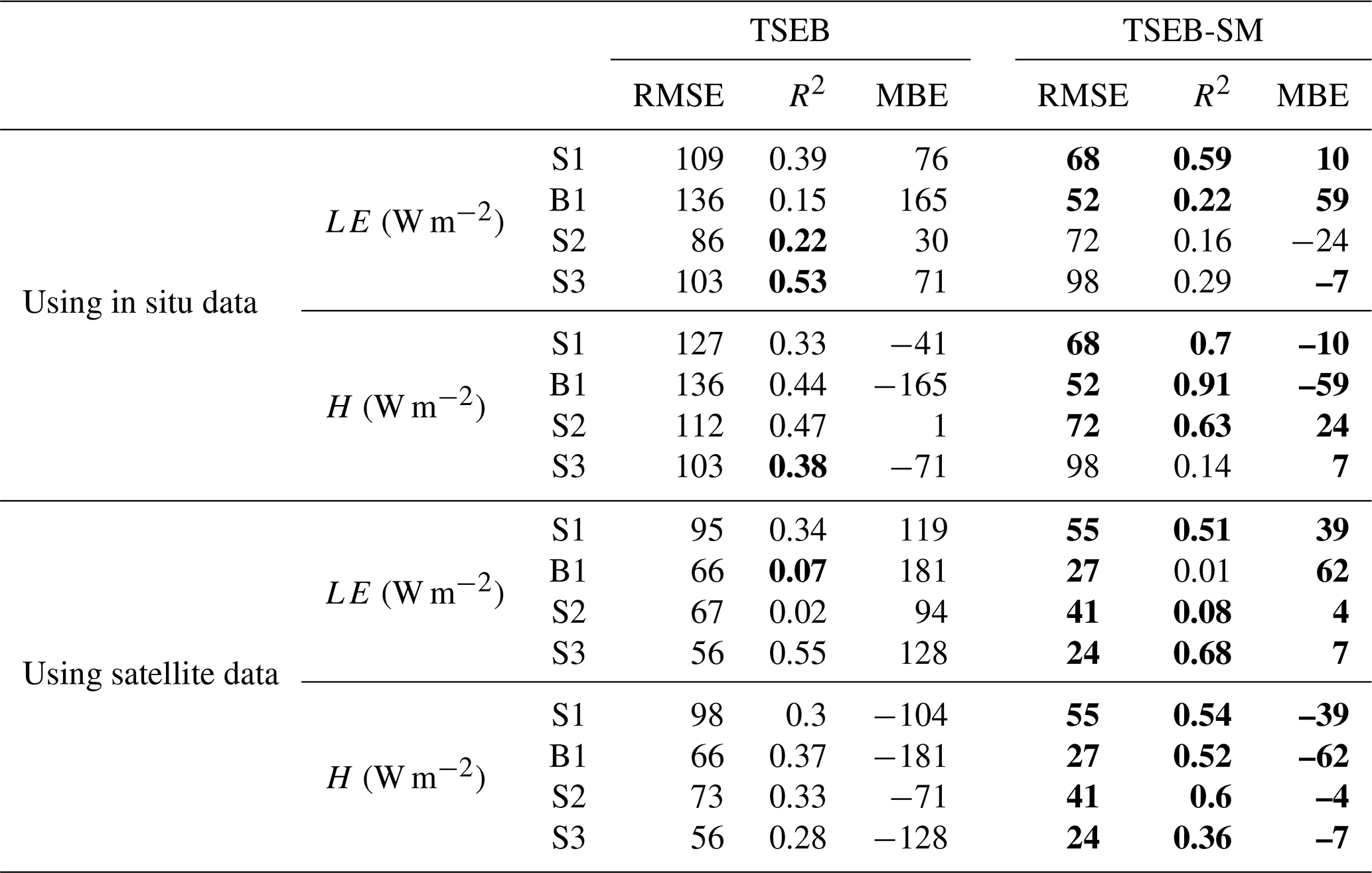
Thermal-based two-source energy balance modeling is essential to estimate the land evapotranspiration (ET) in a wide range of spatial and temporal scales. However, the use of thermal-derived land surface temperature (LST) is not sufficient to simultaneously constrain both soil and vegetation flux components. Therefore, assumptions (about either soil or vegetation fluxes) are commonly required. To avoid such assumptions, an energy balance model, TSEB-SM, was recently developed by Ait Hssaine et al. (2018 b) in order to consider the microwave-derived near-surface soil moisture (SM), in addition to the thermal-derived LST and vegetation cover fraction (f_c) normally used. While TSEB-SM has been successfully tested using in situ measurements, this paper represents its first evaluation in real life using 1 km resolution satellite data, comprised of MODIS (MODerate resolution Imaging Spectroradiometer) for LST and f_c data and 1 km resolution SM data disaggregated from SMOS (Soil Moisture and Ocean Salinity) observations. The approach is applied during a 4-year period (2014–2018) over a rainfed wheat field in the Tensift basin, central Morocco. The field used was seeded for the 2014–2015 (S1), 2016–2017 (S2) and 2017–2018 (S3) agricultural seasons, while it remained unploughed (as bare soil) during the 2015–2016 (B1) agricultural season. The classical TSEB model, which is driven only by LST and f_c data, significantly overestimates latent heat fluxes (LE) and underestimates sensible heat fluxes (H) for the four seasons. The overall mean bias values are 119, 94, 128 and 181 W m⁻² for LE and −104, −71, −128 and −181 W m⁻² for H, for S1, S2, S3 and B1, respectively. Meanwhile, when using TSEB-SM (SM and LST combined data), these errors are significantly reduced, resulting in mean bias values estimated as 39, 4, 7 and 62 W m⁻² for LE and −10, 24, 7, and −59 W m⁻² for H, for S1, S2, S3 and B1, respectively. Consequently, this finding confirms again the robustness of the TSEB-SM in estimating latent/sensible heat fluxes at a large scale by using readily available satellite data. In addition, the TSEB-SM approach has the original feature to allow for calibration of its main parameters (soil resistance and Priestley–Taylor coefficient) from satellite data uniquely, without relying either on in situ measurements or on a priori parameter values.

Download & links

Article (PDF, 1822 KB)

How to cite

How to cite.

Dates

Received: 06 Mar 2019 – Discussion started: 23 Apr 2019 – Revised: 01 Feb 2020 – Accepted: 08 Mar 2020 – Published: 09 Apr 2020

1 Introduction

Evapotranspiration (ET) is a crucial water flux for drought monitoring (Bhattarai et al., 2019; Gerhards et al., 2019; Mallick et al., 2014, 2016, 2018), water resource management (Madugundu et al., 2017; Tasumi, 2019) and climate simulation (Littell et al., 2016; Molden et al., 2010) in the semi-arid ecosystems. A precise estimate of ET determines the crop water requirements, which subsequently allows the optimization of irrigation water applications (Allen et al., 1998).

Regarding the data availability over extended areas, remote sensing is the only viable technique that can provide representative and multi-resolution measurements of ET. As a consequence, the spatial modeling has become a dominant means of estimating ET fluxes over regional and continental areas (Anderson et al., 2007; Fisher et al., 2017). In this context, numerous models based on land surface temperature (LST) data have been developed, such as (i) residual balance methods that consider ET to be the residual term of the energy balance, like TSEB (two-source energy balance, Norman et al., 1995) and SEBS (surface energy balance system, Su, 2002), (ii) contextual methods that estimate ET as the potential ET times the evaporative efficiency (Moran et al., 1994) or as the available energy times the evaporative fraction (Merlin et al., 2013; Roerink et al., 2000) and (iii) other categories of models that integrate LST into a water balance model (Olivera-Guerra et al., 2018) or into the Penman–Monteith energy balance (PMEB) equation to directly estimate ET (Amazirh et al., 2017; Mallick et al., 2015, 2018).

Among well-known temperature-driven energy flux models, the TSEB model proposed by Norman et al. (1995) has been shown to be robust for a wide range of landscapes (Colaizzi et al., 2012; Ait Hssaine et al., 2018 a). TSEB has two key input variables, which can be derived from remote sensing data. The first one is the LST and the second is the vegetation cover fraction (f_c). The TSEB model adopts an iterative procedure, in which an initial estimate of the plant transpiration is given by the Priestly–Taylor (PT) formulation (Priestley and Taylor, 1972). This assumption requires few input data and allows a precise estimate of potential ET (Fisher et al., 2008). Nevertheless, several studies (Ait Hssaine et al., 2018 b; Fisher et al., 2008; Jin et al., 2011; Yang et al., 2015) have stressed that the PT coefficient cannot be considered a constant value, as it is influenced by several parameters. Other authors (Gonzalez-dugo et al., 2009; Long and Singh, 2012; Morillas et al., 2014) reported that the PT approach may overestimate the canopy ET, especially for low soil wetness, and/or sparse vegetation cover, because it does not include a reasonable reduction of the initial canopy ET under stress conditions. Recently, Boulet et al. (2015) developed the Soil-Plant-Atmosphere and Remote Sensing Evapotranspiration (SPARSE) model, which is similar to the TSEB model in its basic assumption but with additional constraints to improve the ET model performance in heterogeneous vegetation. The former first generates an equilibrium LST from the evaporation efficiency and the transpiration efficiency estimates by assuming that their values are equal to 1. Then, LST is implemented in the SPARSE retrieval mode to circumscribe the output fluxes by both limiting cases (namely the fully stressed and potential conditions). In spite of the good retrieval performances of ET by this model, significant uncertainties are observed during the quasi-senescent vegetation period (Boulet et al., 2015).

Alternatively to the use of LST as a proxy for ET, numerous studies have stressed that the soil moisture plays a critical role in the partitioning of available energy into latent and sensible heat fluxes and is the prominent controlling factor of actual ET (Boulet et al., 2015; Gokmen et al., 2012; Kustas et al., 1998, 1999; Li et al., 2006). Several authors have revised the well-known LST-based TSEB model and replaced the LST with microwave-derived surface soil moisture (SM) to estimate daily ET (Bindlish et al., 2001; Kustas et al., 1998, 1999; Li et al., 2006). Bindlish et al. (2001) found that the impact of SM on surface fluxes is strongly related to the vegetation cover. The impact is high for low fraction cover and relatively weak for the high cover fraction. Moreover, the soil evaporation is constrained by the SM through its soil-texture-dependent coefficients (a_rss and b_rss) reported in Sellers et al. (1992). In the same way, Li et al. (2006) indicated that the model performance is sensitive to these two coefficients, and thus they proposed averaging the output of LST-based TSEB and SM-based TSEB models in order to provide more consistent results over a wide range of conditions.

Previous studies, either LST- or SM-based, agree with the view that combining both LST and SM information at a time would enhance the robustness and accuracy of ET estimates in various biomes and climates. Nevertheless, few studies have simultaneously combined both observations in a unique energy balance model. One difficulty lies in developing a consistent representation of the soil evaporation (as constrained by SM, Chanzy and Bruckler, 1993), the total ET (as constrained by LST, Norman et al., 1995) and the plant transpiration (as indirectly constrained by both LST and SM, Ait Hssaine et al., 2018 b).

Gokmen et al. (2012) explicitly integrated the SM derived from AMSR-E (Advanced Microwave Scanning Radiometer for EOS) data (Owe et al., 2008) into the LST-derived SEBS model via the kB−1 parameter, which plays an important role in the aerodynamic resistance. The updated SEBS model (SEBS-SM) provided a large improvement of sensible heat flux and thus ET estimates under water-limited conditions. The point is that the soil evaporation reduction parameters were calibrated using in situ measurements, which limits the validity of the approach over large areas. In the same vein, Gan and Gao (2015) incorporated a SM-based soil resistance term in the TSEB formalism and calibrated several parameters (including the PT coefficient) using LST data. The obtained results showed that the model calibrated by LST data performed better than the non-calibrated one. Note that the parameters of the soil resistance were set to constant values as in Sellers et al. (1992) and Li et al. (2006). As a further step towards the combination of LST and SM data, Ait Hssaine et al. (2018 b) modified the TSEB formalism (Kustas and Norman, 1999; Norman et al., 1995) (named TSEB-SM) and proposed a new calibration strategy of the main PT-based TSEB-SM parameters. The TSEB-SM model was tested using in situ measurements and provided an important improvement in terms of latent heat flux/sensible heat flux estimates compared to the classic TSEB all along the agricultural season, especially during the crop emergence and the senescence periods. Such improvements are attributed to stronger constraints exerted on the representation of soil evaporation (via SM data and the calibrated soil parameters) and plant transpiration (via the calibrated daily PT coefficient). It should be noted that only LST and SM data are used for the calibration of yearly a_rss and b_rss as well as daily α_PT, while the flux measurements are needed only for the validation of the TSEB-SM-simulated sensible and latent heat fluxes.

One crucial point is that all the above studies based on remotely sensed SM and LST have neglected the mismatch in the spatial resolutions of readily available SM products. Especially the global-scale SM data sets have a typical resolution of 40–50 km (Entekhabi et al., 2010; Kerr et al., 2010; Njoku et al., 2003). Such spatial resolution is generally unsuitable or even incompatible with many hydrological and agricultural applications. To fill the gap, disaggregation approaches of AMSR-E, SMOS (Soil Moisture and Ocean Salinity) and SMAP (Soil Moisture Active and Passive) like SM data have been developed (Peng et al., 2017) but, to date, there has been no application of SM-based ET models to disaggregate SM data sets. In addition, the use of remote sensing data would be necessary in order to avoid the time-consuming process of calibrating the TSEB model over each field.

Although TSEB-SM has the capability to calibrate its main parameters from remotely sensed data, the real-life application needs extensive evaluation and testing. The objective of this paper is thus to demonstrate for the first time this capacity using disaggregated SMOS and MODIS (MODerate resolution Imaging Spectroradiometer) data. For this purpose, TSEB-SM is applied to 1 km resolution using MODIS LST∕f_c data and to SMOS SM data. To make the SMOS data spatially consistent with MODIS data, the SMOS SM is disaggregated at 1 km resolution using the DisPATCh (DISaggregation based on Physical And Theoretical scale Change) algorithm (Malbéteau et al., 2016; Merlin et al., 2013; Molero et al., 2016). The proposed methodology is evaluated over a rainfed wheat field in the Tensift basin, central Morocco during four agricultural seasons (2014–2018).

2 Data description and methods

2.1 Site and in situ data description

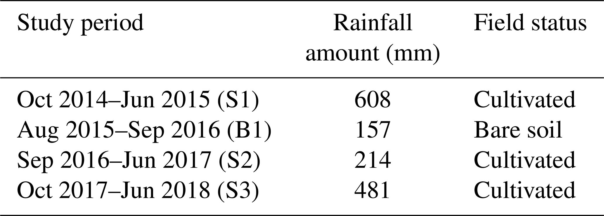
The study site is situated in the east (Sidi Rahal) of the Tensift basin in central Morocco (see Fig. 1). The region is characterized by a semi-arid Mediterranean climate, with an average yearly precipitation of about 250 mm and an atmospheric evaporative demand around 1600 mm yr⁻¹ according to the FAO method (Allen et al., 1998; Jarlan et al., 2015). Soil is characterized by a fine texture with 47 % of clay, 33 % of loam and 18.5 % of sand (Er-Raki et al., 2007). The experiment has been set up in a rainfed wheat (“Bour”) field since 2013 (Ali Eweys et al., 2017; Amazirh et al., 2018; Merlin et al., 2018). Located within a larger area occupied by rainfed wheat “Bour”, this field was chosen to be representative at a scale of 1 km, thus enabling the comparison between 1 km resolution satellite-derived and localized in situ measurements. The field was seeded in September 2014, September 2016 and September 2017 for the 2014–2015 (S1), 2016–2017 (S2) and 2017–2018 (S3) agricultural seasons, respectively. However, it was not ploughed (remained as bare soil) during the 2015–2016 (B1) agricultural season due to an unusual lack of precipitation in autumn–winter 2015 (Merlin et al., 2018) (Table 1).

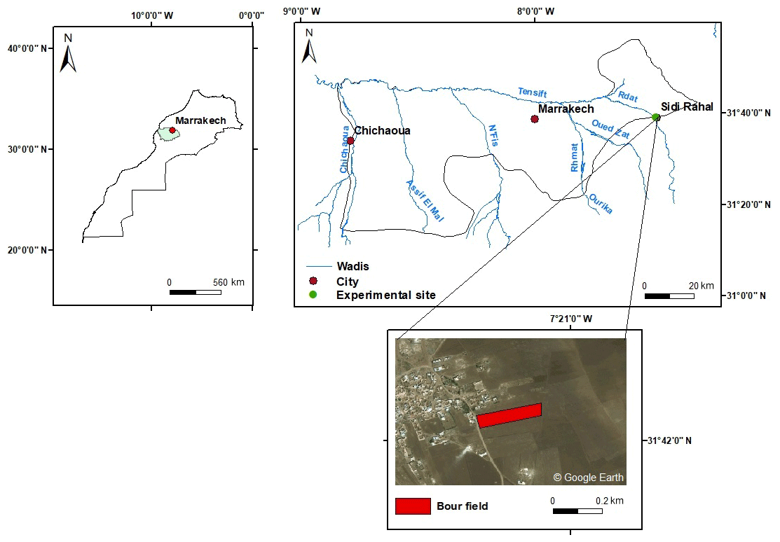
https://www.hydrol-earth-syst-sci.net/24/1781/2020/hess-24-1781-2020-f01

Figure 1Location of the Sidi Rahal site (east of Marrakech) in the Tensift basin, central Morocco.

Table 1Characteristics of the study site.

Download Print Version | Download XLSX

The field was instrumented by an eddy covariance (EC) system at a 2 m height. EC tower includes a CSAT3 3-D sonic anemometer that measures the wind and temperature fluctuations and a krypton hygrometer, KH20, that measures the concentration of water vapor. The EC tower is also equipped with a CNR1 radiometer (Kipp and Zonen) to measure the four components of the net radiation (R_n) with several heat flux plates (HFT3-L, Campbell Scientific Ltd) to measure the soil heat flux (G). Energy balance closure analysis indicated that the available energy (R_n−G) was generally higher than the EC measurements. The relative closure was about 68 %, 76 %, 79 % and 79 % for S1, S2, S3 and B1, respectively. The sensible and latent heat fluxes (H and LE) were finally corrected to force the closure of the energy balance by the Bowen ratio method (Twine et al., 2000). LST is measured at the EC station by using two Apogee IRTS-P infrared radiometers, oriented downward and measuring the surface-leaving radiance between 8 and 14 µm, set up at a 2 m height above the ground. An estimate of LST is obtained by averaging both measurements. The soil water content is measured at various depths (5, 10, 20, 30, 50, 70 cm) using Time Domain Reflectometry probes (model CS616) installed in a soil pit at the bottom of the EC tower. A weather station was set up nearby the studied field to measure air temperature, solar radiation, relative humidity, wind speed and rainfall at a 30 min time step.

2.2 Remote sensing data

2.2.1 MODIS

Three products from the MODIS sensor onboard the Terra and Aqua satellites are used in this study: the (1) MODIS Terra/Aqua Land Surface Temperature product (MOD11A1/MYD11A1), the (2) MODIS Terra Vegetation Indices product (MOD13A2) and the (3) MODIS Albedo (combined Terra and Aqua) product (MCD43A3). All products are gridded in the sinusoidal projection.

The MOD11A1 and MYD11A1 provide LST at 1 km spatial resolution under clear-sky conditions, derived from Terra and Aqua, respectively. Brightness temperatures from bands 31 and 32 are used to derive LST through a generalized split-window algorithm. The MOD13A2 provides several vegetation indices at 1 km resolution. One particular vegetation index of interest in this study is NDVI, available at 16-day temporal intervals. This product is derived from bands 1 and 2 of the MODIS Terra satellite.

The obtained NDVI is used to derive the leaf area index (LAI) via the following formulation (Wang et al., 2013):

\begin{matrix} (1) & LAI = {(NDVI \times \frac{1 + NDVI}{1 - NDVI})}^{1 / 2} . \end{matrix}

The vegetation cover fraction is expressed as (Kustas and Norman, 1997)

\begin{matrix} (2) & f_{c} = 1 - \exp (- 0.5 LAI) . \end{matrix}

Finally, the MCD43A3 product provides the surface albedo (α) at 500 m resolution every 16 d. The latter is generated from both the Terra and Aqua products. In this work, the shortwave broadband α is used by integrating its value over the entire solar emission spectrum (0.3–5.0 µm). This value is obtained as a weighted average of the directional hemispherical reflectance (black-sky-α) and the bi-hemispherical reflectance (white sky α) using their two extreme values. The current α (called “blue sky”) is a weighted average between these two extreme cases (Lewis and Barnsley, 1994). Herein, the percentages of 85 % and 15 % are used for the direct and diffuse lights, respectively.

2.2.2 SMOS

The SMOS mission measures the natural (passive) microwave radiation around the frequency of 1.4 GHz (L-band). It aims to monitor SM at a depth of about 3–5 cm with a spatial resolution of about 40 km and an accuracy better than 0.04 m³ m⁻³ (Kerr et al., 2012). The revisiting time at the Equator is 3 d for both ascending and descending passes, which are Sun synchronous at 06:00 and 18:00 LT, respectively. The SMOS level-3 1 d global SM product (MIR CLF31A/D) posted on the ∼25 km Equal Area Scalable Earth (EASE) version 1.0 grid is used as input to the DisPATCh algorithm.

2.2.3 DisPATCh

The DisPATCh remote sensing algorithm combines the coarse-scale microwave-retrieved SM with high-resolution optical/thermal data within a downscaling relationship to produce SM at a higher spatial resolution.

Soil (T_s,min, T_s,max) and vegetation (T_v,min, T_v,max) temperature endmembers are estimated from the polygon obtained by plotting MODIS LST against MODIS NDVI, where the LST is partitioned into its soil and vegetation components according to the trapezoid method of Moran (Moran et al., 1994). Details on the DisPATCh algorithm and the methodology to determine dry and wet edges can be found in Merlin et al. (2012). The retrieved soil temperature is then used to estimate the soil evaporative efficiency (SEE), which is defined as the ratio of actual to potential soil evaporation. Finally, DisPATCh converts the high-resolution optically derived SEE fields into high-resolution SM fields given a semi-empirical SEE model and a first-order Taylor series expansion around the SMOS observation. In our application, we applied DisPATCh to 40 km resolution SMOS level-3 SM and 1 km resolution MODIS optical/thermal data to produce SM at a 1 km resolution (Molero et al., 2016). The input data sets are composed of MODIS LST, MODIS NDVI and the GTOPO digital elevation model (DEM) used to correct LST for topographic effects (Malbéteau et al., 2016; Merlin et al., 2013).

2.3 Methods

2.3.1 TSEB-SM

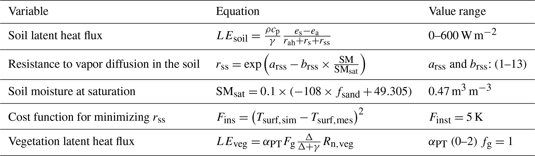
The recently developed TSEB-SM is fully described in Ait Hssaine et al. (2018 b). The equations and sub-equations used in TSEB-SM are provided in Table 2; the main equations are given below. The originality of TSEB-SM is to integrate SM observations in addition to LST and vegetation cover fraction data in order to calibrate both the soil resistance to evaporation (constant parameters) and the PT coefficient on a daily basis. The model is based on the original TSEB formalism, meaning that the energy balance for vegetation is the same as in TSEB using the PT formula, although the soil evaporation is estimated as a function of SM using a soil resistance developed by Sellers et al. (1992). The use of the soil resistance formulation is justified by the fact that its main parameters (a_rss, b_rss) can be adjusted based on soil texture characteristics (Merlin et al., 2016) or by combining SM and LST data under bare (Merlin et al., 2018) or partially covered (Ait Hssaine et al., 2018 b) soil conditions.

Table 2Mean equations of TSEB-SM.

Download Print Version | Download XLSX

The surface soil heat flux is estimated as a fraction of R_n,soil:

\begin{matrix} (3) & G = c_{g} \cdot R_{n, soil}, \end{matrix}

where c_g∼0.35 (Choudhury et al., 1987).

The vegetation latent heat flux LE_veg is estimated via the PT formulation:

\begin{matrix} (4) & L E_{veg} = α_{PT} \cdot f_{g} \cdot \frac{△}{△ + γ} \cdot R_{n, veg}, \end{matrix}

where α_PT is the PT coefficient, f_g the fraction of green vegetation, γ the psychometric constant (≈67 Pa K⁻¹), △ the slope of the relationship between saturation vapor pressure and air temperature, and R_n,veg the vegetation net radiation. Note that f_g is set to 1 as the α_PT coefficient is varied (through the calibration procedure) to take into account the fraction of transpiring vegetation. The soil latent heat flux is estimated using the resistance formulation:

\begin{matrix} (5) & L E_{soil} = \frac{ρ c_{p}}{γ} \frac{e_{s} - e_{a}}{r_{ah} + r_{s} + r_{ss}}, \end{matrix}

where e_s is the saturated vapor pressure at the soil surface, e_a the actual air vapor pressure, r_ah the aerodynamic resistance calculated from the adiabatically corrected logarithmic temperature profile equation (Brutsaert, 1982) and r_s the surface-soil resistance to transport of heat between the soil surface and a height representing the canopy estimated using (Sauer et al., 1995). Both resistances are simulated every 30 min (between 11:00 and 14:00 LT) and at Terra and Aqua overpass times for in situ and satellite data, respectively. r_ss is computed as a function of SM and is expressed as (Chirouze et al., 2014; Li et al., 2006; Sellers et al., 1992)

\begin{matrix} (6) & r_{ss} = \exp (a_{rss} - b_{rss} \times \frac{SM}{{SM}_{sat}}), \end{matrix}

with SM being the 0–5 cm SM, a_rss and b_rss are two empirical parameters (to be calibrated) and SM_sat is the SM at saturation expressed as (Cosby et al., 1984)

\begin{matrix} (7) & {SM}_{sat} = 0.1 \times (- 108 \times f_{sand} + 49.305), \end{matrix}

with f_sand being the sand percentage of soil.

In Ait Hssaine et al. (2018 b), an innovative calibration approach of α_PT, a_rss and b_rss is developed from in situ SM and LST data (Ait Hssaine et al., 2018 b). The calibration methodology is briefly explained below.

Retrieval and calibration of r_ss, a_rss and b_rss

The r_ss is first adjusted by minimizing a cost function defined by

\begin{matrix} (8) & F_{inst} = {(T_{surf, sim} - T_{surf, mes})}^{2}, \end{matrix}

with T_surf,sim and T_surf,mes being the simulated and measured LST, respectively.

The T_surf,sim was simulated as follows:

\begin{matrix} (9) & T_{surf, sim} = {(f_{c} \cdot {(T_{veg})}^{4} + (1 - f_{c}) \cdot {(T_{soil})}^{4})}^{0.25}, \end{matrix}

where T_veg and T_soil are the vegetation and soil components of temperature (K). The LST is simulated every 30 min (between 11:00 and 14:00 LT) and at Terra and Aqua overpass times for in situ and satellite data, respectively. The LST at the first calibration step is simulated with a constant value of α_PT (average value of the α_PT retrieved for f_c>0.5). Then, for the second calibration step, it is simulated using the daily retrieved α_PT.

The inverted r_ss is then correlated with the SM (in situ or DisPATCh) to determine the a_rss and b_rss parameters by considering that, when f_c is lower than a given threshold (f_c,thres), the dynamics of total LE is mainly controlled by the temporal variation of soil evaporation, meaning that both soil parameters are estimated when the PT coefficient can be set to a constant value.

Daily α_PT retrieval

Once both parameters a_rss and b_rss have been estimated, the PT coefficient is retrieved on a daily basis when f_c is larger than f_c,thres, by minimizing a cost function at the Terra and Aqua-MODIS overpass times:

\begin{matrix} (10) & F_{daily} = \sum {(T_{surf, sim} - T_{surf, mes})}^{2} . \end{matrix}

In fact, an iterative loop is run on soil (r_ss) and vegetation (α_PT) parameters to reach convergence of all parameters. LST and SM data are thus used for calibration, while the calibrated TSEB-SM is run on a daily basis using SM data as forcing solely (in addition to vegetation cover fraction data). In this paper, an improvement is made on the former version of TSEB-SM to normalize the output fluxes using the LST-derived available energy. Therefore, the new version of TSEB-SM uses both LST and SM data (in addition to vegetation cover fraction data) as forcing on a daily basis. In practice, the latent and sensible heat fluxes derived from the TSEB-SM model are re-computed using the TSEB-SM derived evaporative fraction (EF, defined as the ratio of latent heat to available energy) and the LST-derived available energy. The rationale is that numerous modeling studies have shown the regularity and constancy of EF during daylight hours in cloud-free days (Gentine et al., 2011; Lhomme and Elguero, 1999; Shuttleworth et al., 1989) and the EF has a strong link with SM availability (Bastiaanssen and Ali, 2003), which is an important factor for estimating latent heat flux. For that purpose, the LST data collected at the Terra and Aqua-MODIS overpass times are used to estimate the instantaneous R_n and G. A ratio between the daily (obtained as an average value between Aqua and Terra overpass times) latent heat flux LE_daily and the daily available energy ( $R_{n, daily} - G_{daily}$ ) is used to calculate an average daily EF:

\begin{matrix} (11) & EF = \frac{L E_{daily}}{R_{n, daily} - G_{daily}} . \end{matrix}

The daily EF and the instantaneous available energy (calculated using Terra and Aqua MODIS LST) are finally used to re-calculate the instantaneous TSEB-SM output of LE and H by the following formulas:

\begin{array}{l} (12) & L E = EF \times (R_{n} - G), \\ (13) & H = (1 - EF) \times (R_{n} - G) . \end{array}

2.3.2 Uncertainty in TSEB-SM input data

The LST collected by MODIS at Terra and Aqua overpass times and the SM product derived at 1 km resolution from the DisPATCh algorithm applied to SMOS data are used as input to TSEB and TSEB-SM models. Validation of TSEB and TSEB-SM input data prior to the evaluation of model output is an important issue, because of the scale discrepancy between the spatial resolution (1 km) of MODIS/DisPATCh data and the footprint of the EC flux measurements that does not exceed 100 m (Schmid, 1994).

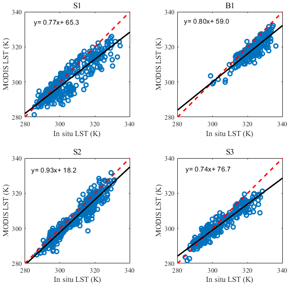
https://www.hydrol-earth-syst-sci.net/24/1781/2020/hess-24-1781-2020-f02

Figure 2Scatterplots of MODIS versus in situ LST at the Sidi Rahal site for the S1 (2014–2015), B1 (2015–2016), S2 (2016–2017) and S3 (2017–2018) agricultural seasons, separately, (red dashed line is the 1:1 line; black line is the regression line).

Download

Several studies have demonstrated the effectiveness of DisPATCh 1 km resolution SM. Malbéteau et al. (2016) compared DisPATCh SM data with the in situ measurements collected in the Murrumbidgee catchment in southeastern Australia. Their results showed that DisPATCh improved the spatial representation of SM at 1 km resolution (compared to the original 40 km resolution SMOS SM), especially in semi-arid areas. Recently, Malbéteau et al. (2018) combined the DisPATCh SM over the entire year 2014 (Sidi Rahal, Morocco) with the continuous predictions of a surface model in order to obtain a better estimate of daily SM at 1 km resolution. They found that the assimilation of DisPATCh data improved quasi-systematically the dynamics of SM.

Figure 2 shows the scatterplots of MODIS LST (at Terra and Aqua overpass) versus in situ measurements for the four agricultural seasons separately. The obtained R², root mean square error (RMSE), and mean bias error (MBE) are reported in Table 3. The statistical comparison shows strong linear correlations ( $0.76 \leq R^{2} \leq 0.90$ ) for all years. The RMSE is around 4 K for the S2 (2016–2017) and S3 (2017–2018) agricultural seasons, while it reaches 6 K for S1 (2014–2015) and B1 (2015–2016), respectively. The observed scatter may stem from the fact that the localized (1 or 2 m wide) in situ LST is not fully representative of the 1 km resolution MODIS pixel (Ait Hssaine et al., 2018 a; Yu et al., 2017). For all years (S1–3, B1), it can be seen that the MBE is negative. Note that the MBE is the greatest when the temperatures are largest. Such a systematic error is probably due to the non-representativeness of the in situ LST observations when compared to the corresponding scale of MODIS observations.

Table 3Validation results of DisPATCh SM and MODIS LST at the Sidi Rahal site.

Download Print Version | Download XLSX

https://www.hydrol-earth-syst-sci.net/24/1781/2020/hess-24-1781-2020-f03

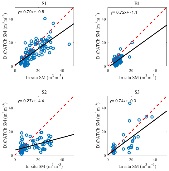
Figure 3Scatterplots of the 1 km resolution DisPATCh versus in situ SM at the Sidi Rahal site for the S1 (2014–2015), B1 (2015–2016), S2 (2016–2017) and S3 (2017–2018) agricultural seasons, separately.

Download

The DisPATCh products have been extensively evaluated, especially over semi-arid areas like the Marrakech region (Bandara et al., 2015; Colliander et al., 2017; Djamai et al., 2015; Escorihuela and Quintana-Seguí, 2016; Escorihuela et al., 2018; Lievens et al., 2015; Malbéteau et al., 2016, 2018; Merlin et al., 2012, 2013, 2015; Molero et al., 2016; Ojha et al., 2019; Peng et al., 2017; Sabaghy et al., 2020). Actually, the scatterplots of Fig. 3 aim to verify that the DisPATCh soil moisture is consistent, during four agricultural seasons (S1, B1, S2 and S3), at the site level where the comparison between TSEB and TSEB-SM is undertaken. The statistical results including the coefficient of determination (R²), the RMSE, and the MBE are reported in Table 3. The R² ranges from 0.27 to 0.55, the RMSE from 0.04 to 0.09 m³ m⁻³ and the MBE from −0.05 to −0.03 m³ m⁻³. These results are encouraging considering the heterogeneous land use composed of rainfed wheat, bare soil, and fallow and farm building (see Fig. 4). In fact, the localized in situ measurements may not be perfectly representative of the 1 km resolution satellite data. Note that the efficiency of DisPATCh is supposedly higher for low SM values (Malbéteau et al., 2016), which is clearly illustrated during the B1 season, while it is lower for high SM values (after rain events). This can be explained by the constraints of atmospheric and vegetation conditions on disaggregation results as well as the saturation of SEE in the higher SM range. Another major issue that can lead to differences between DisPATCh and in situ SM is that the ground SM sensors are buried at a depth of 5 cm, while the penetration of the L-band wave varies between 2 and 5 cm depending on soil conditions (notably SM content, texture). For S2, the SM provided by DisPATCh underestimated field measurements, especially in the higher SM range. This particular behavior could be explained by the particularly low precipitation amount during this year. It is especially possible that the surrounding plots were not sown by neighboring farmers, resulting in a soil that dried quickly compared to our field, which retained the SM for a longer period of time.

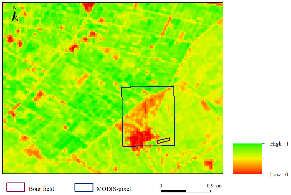
https://www.hydrol-earth-syst-sci.net/24/1781/2020/hess-24-1781-2020-f04

Figure 4NDVI image derived from Landsat data acquired on 17 April 2018. The experimental field and the overlaying 1 km resolution MODIS pixel are superimposed.

Download

Note that despite the relative heterogeneity within the 1 km pixel (characterized by rainfed wheat in addition to bare soil and fallow), the comparison between field measurements and 1 km resolution satellite data reflects acceptable accuracies.

3 Results and discussion

In this section, the a_rss and b_rss parameters and the α_PT are firstly retrieved by following the two-step calibration based on a threshold of f_c (cited in the Methods section). Then, the obtained calibrated values are used to estimate the surface fluxes using TSEB-SM. Finally, TSEB-SM fluxes are evaluated against the eddy covariance measurements, and results are compared with the original TSEB. To facilitate the interpretation of the simulation results using MODIS and SMOS/DisPATCh data as input, the calibration and validation steps are previously tested using in situ (LST and SM) data.

3.1 Retrieving a_rss and b_rss parameters

The soil resistance r_ss is inverted for $f_{c} \leq f_{c, thres}$ between 11:00 and 14:00 LT and at the Terra and Aqua overpass time step for in situ and satellite data, respectively. The result of this inversion is correlated with the actual to saturated soil moisture ratio SM∕SM_sat to determine a_rss and b_rss parameters. The calibration process is applied for each season independently. Then a pair (a_rss, b_rss) is calculated for the entire study period for in situ and satellite data, respectively.

Figure 5a and b plot the ln (r_ss) versus in situ SM∕SM_sat using in situ and satellite data, respectively. The mean retrieved values (7.62, 2.43) and (7.32, 4.58) for in situ and satellite data, respectively, are close to the values found in Li et al. (2006) (8.2, 4.3) and in Ait Hssaine et al. (2018 b) (7.2, 4). However, by comparing both figures (Fig. 5a and b), one notes that the use of in situ data generates more scatter than with satellite data. The apparent scatter in retrieved r_ss could be interpreted by the impact of the daily cycle of meteorological (evaporative demand) conditions or soil property differences (Merlin et al., 2011, 2016, 2018). The retrieved soil parameters also vary from year to year: the standard deviation is 0.39 and 1.69 for a_rss and b_rss, respectively. This can be explained by the compensation effects linking a_rss and b_rss parameters which prove the empirical nature of the r_ss. Another major issue that can lead to these differences is the depth of SM measurements (Merlin et al., 2011). In Sellers et al. (1992), the near-surface soil moisture is defined in the 0–5 cm soil layer, whereas in our field, SM measurements are made at 5 cm depth. Also, the sensing depth of SMOS observations is generally shallower than the in situ surface measurements (Escorihuela et al., 2010). Moreover, the variability of a_rss and b_rss in Fig. 5b using remote sensing data can be linked to the scale difference between DisPATCh SM/MODIS products (1 km) and the field measurements. As shown in Fig. 3, the field is surrounded by trees, buildings and fallows, which causes the spatial heterogeneity within the pixel of 1 km. This heterogeneity can introduce errors into the model inversion. Nevertheless, soil parameters are quite similar for in situ and satellite data sets. Therefore, the heterogeneity issues within the 1 km pixel scale are minor in this study.

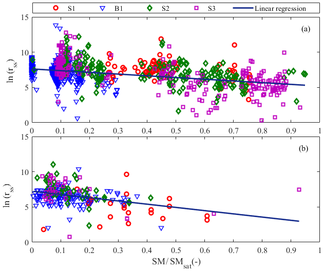
https://www.hydrol-earth-syst-sci.net/24/1781/2020/hess-24-1781-2020-f05

Figure 5ln (r_ss) versus SM/SM_sat (calibration step 1) using in situ (a) and satellite (b) data.

Download

3.2 Time series of daily retrieved α_PT

The second calibration step consists in inverting the daily α_PT when vegetation is covering a significant part of soil ( $f_{c} > f_{c, thres}$ ), for the three seasons of rainfed wheat (S1–S3), by using in situ data and satellite data, separately. Herein, the calibration of α_PT is bounded by minimum (0) and maximum (2) acceptable physical values, in order to avoid unacceptable values of α_PT that can be produced because of the uncertainties in daily LST estimates. Such an upper bounding is especially needed when vegetation partially covers the soil.

3.2.1 Using in situ data

Figure 6 plots the daily variation of α_PT for each season (S1–S3) separately, using in situ data. The mean retrieved values of α_PT are 1.26, 1.12 and 1.09 for S1, S2 and S3, respectively. In all cases, the mean α_PT is close to the theoretical α_PT value (1.26). It is well observed that the retrieved α_PT for S1 is slightly larger compared to those obtained for both S2 and S3. This can be explained by the timing and amount of rainfall during each season. Note that unexpected low values of α_PT are recorded for S3 during the first few days (25 January–4 March) of the development stage. They may be associated with uncertainties in retrieved α_PT, as the impact of soil surface is still significant, as well as with a relatively low evaporative demand especially since this period coincides with cloudy days and abundant precipitations. Indeed, the coupling between transpiration (and hence retrieved α_PT) and LST is expected to be lower under lower atmospheric demand.

https://www.hydrol-earth-syst-sci.net/24/1781/2020/hess-24-1781-2020-f06

Figure 6Time series of daily retrieved and smoothed α_PT (calibration step 2 – using in situ data and satellite data) collected during S1, S2 and S3.

Download

The retrieved α_PT is then smoothed as in Ait Hssaine et al. (2018 b) to remove outliers and to reduce uncertainties at the daily timescale. The smoothed values of α_PT range from 0 to 1.54, 0 to 1.38 and 0.45 to 1.43 for S1, S2 and S3, respectively. The maximum of α_PT is close to 1.26 for S2, while it is higher for S1 and S3. This result is in accordance with the total rainfall amounts, which were about 608, 214 and 421 mm for S1, S2 and S3, respectively. Additionally, one can state that the stability of α_PT strongly depends on the rainfall distribution along the agricultural season. The daily α_PT is more stable for S1 than for S2 and S3. Indeed, the amount of rain during S1 is very important, with two peaks of about 83 mm that occurred at the beginning of the season and during the growing stage. The second one coincides exactly with the maximum value of the retrieved α_PT. However, different results are obtained for S2 compared to S1 due to the lowest precipitation amount recorded over that season. As shown in Fig. 6, the amount of rain is concentrated at the beginning of the growing stage (mid December), when the α_PT peaks. Afterward, the smoothed α_PT tends to decrease because of insufficient soil water reserve in the root zone to enable wheat to continue growing. Rainfall is also significant for S3, and every rainfall event causes an immediate (daily) response of α_PT (after 4 March). As mentioned before, the significant error in α_PT retrievals for S3 between 25 January and 4 March induces strong uncertainties in the smoothing function estimates.

3.2.2 Using satellite data

Figure 6 also illustrates the daily variation of α_PT retrieved from satellite data for each season separately. S1 and S2 have a very similar distribution of the retrieved α_PT as compared to the retrieved α_PT using in situ data, respectively. For S3, only six retrieved α_PT values are available because of the non-availability of MODIS products during cloudy days. For this reason, no information linked to the variability of α_PT can be derived during this season. The retrieved values are smoothed and superimposed with the rainfall events. It is clearly shown that the smoothed α_PT for S1 and S2 have the same shape with a small variability when compared with the smoothed α_PT using in situ data, resulting in an error estimated as the RMSE to the mean α_PT ratio, of about 11 % and 19 %, for S1 and S2, respectively. For S1 the maximum of smoothed α_PT is reached at the same time as when using the in situ data, with a value of about 1.38, while the maximum for S2 is reached 10 d before the maximum of the α_PT derived from in situ data with little response of α_PT to rainfall events. These differences may be linked to uncertainties in disaggregated SMOS SM as well as to the weaker availability of satellite data. Because of the small number of data points (retrieved α_PT) during S3, the smoothed α_PT remains at a mostly constant value (∼0.7) throughout the study period, with a significant relative difference of about 34 % when compared with the α_PT retrieved using in situ data.

3.2.3 Interpretation of α_PT variabilities

Figure 7 plots variation of calibrated daily α_PT, superimposed with NDVI and rainfall events. It is visible that the maximum value of NDVI appears sooner than the maximum value of α_PT for both S1 and S3. Such a delay is attributed to the high soil moisture level in the root zone during the maturity stage. Later in the season, α_PT decreases as NDVI starts to decline at the onset of senescence. In contrast, the maximum value of NDVI appears later than the maximum value of α_PT for S2. This can be explained by the fact that rainfall at the beginning of the development phase satisfies the plant requirements, while the rainfall amount during the development stage is relatively low compared to the crop water needs (Kharrou et al., 2011). Large variations in α_PT occur during the agricultural season, as a result of the amount, frequency, and distribution of rainfall along the season. In general, the analysis of the α_PT variability using satellite data illustrates the robustness of the proposed approach, which combines microwave and optical/thermal data to retrieve a water stress indicator at the daily timescale.

https://www.hydrol-earth-syst-sci.net/24/1781/2020/hess-24-1781-2020-f07

Figure 7Time series of calibrated daily α_PT (red – using in situ data, green – using satellite data) superimposed with NDVI and the rainfall events during S1, S2 and S3, separately.

Download

3.3 Surface fluxes

The robustness of TSEB and TSEB-SM for partitioning (R_n−G) into H and LE is evaluated using in situ and remotely sensed LST, SM, and NDVI, separately, at Terra and Aqua MODIS overpasses.

3.3.1 Using in situ data

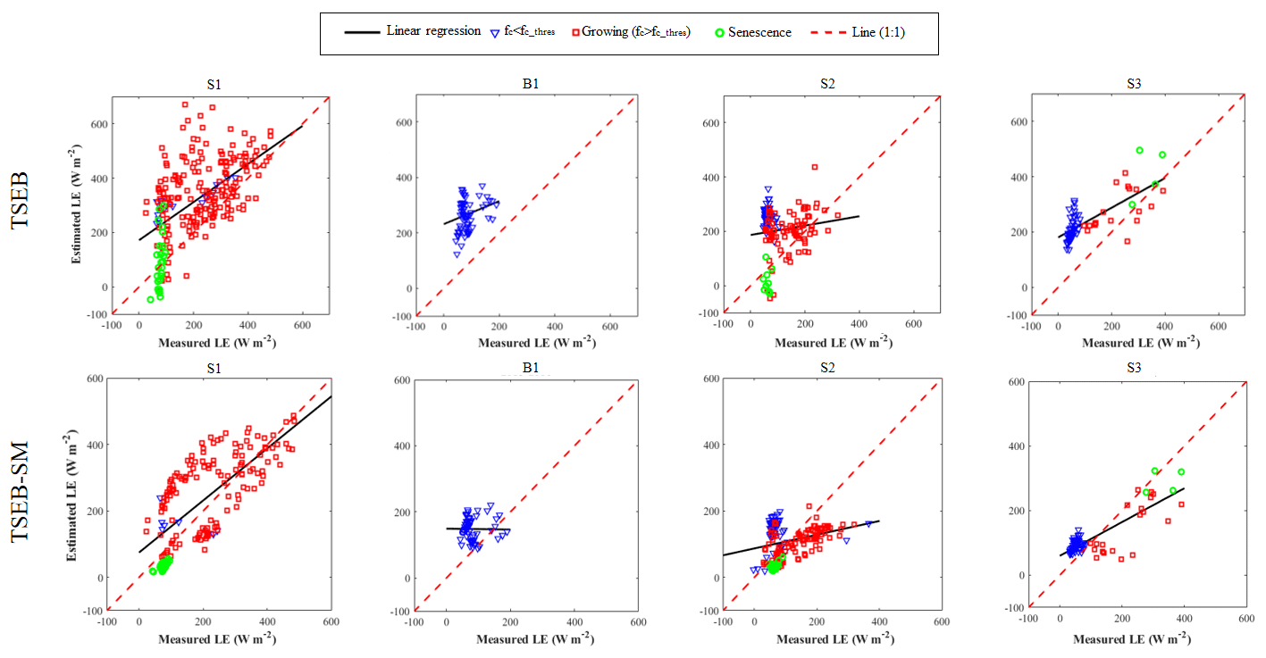
Figure 8 shows an intercomparison of simulated and observed LE for the four seasons separately. TSEB-SM clearly provides improved results compared to the original TSEB. The obtained values of RMSE by TSEB-SM are about 68 and 72 W m⁻² for S1 and S2, respectively, which is significantly lower than those revealed by TSEB (109 and 86 W m⁻², respectively) (see Table 4). For B1 (season of bare soil), TSEB largely overestimates LE with a MBE of about 165 W m⁻² compared to TSEB-SM, which yields a MBE of 59 W m⁻². This overestimation of TSEB is most probably related to an inadequate value of α_PT (=1.26) for bare soil surfaces. In fact, 1.26 is an optimum value for the potential transpiration rate (Agam et al., 2010; Chirouze et al., 2014). In the case of TSEB-SM, biases are reduced thanks to the calibration of the r_ss resistance. Additionally, according to TSEB-SM assumptions, α_PT for f_c≤0.5 is set to the average value of the α_PT retrieved for f_c>0.5. During the B1 season (bare soil conditions), α_PT was hence obtained as an average value of the mean α_PT retrieved for all seasons S1, S2 and S3 when f_c>0.5 (α_PT∼1). However, this value remains relatively high for a bare soil, which yields a slight overestimate of LE measurements (see the B1 case in Fig. 8).

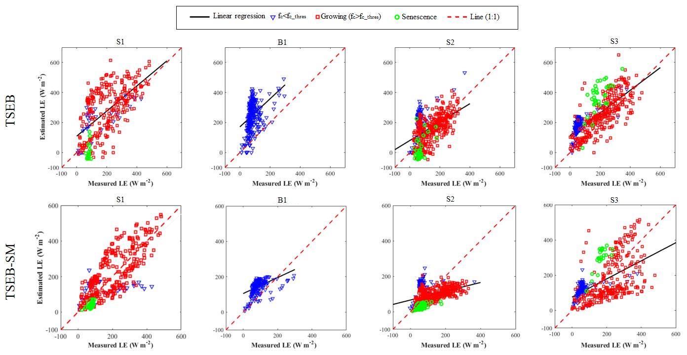
https://www.hydrol-earth-syst-sci.net/24/1781/2020/hess-24-1781-2020-f08

Figure 8Scatterplot of simulated versus observed LE for (top panels) TSEB and (bottom panels) TSEB-SM models using in situ data collected during S1, B1, S2 and S3, respectively.

Download

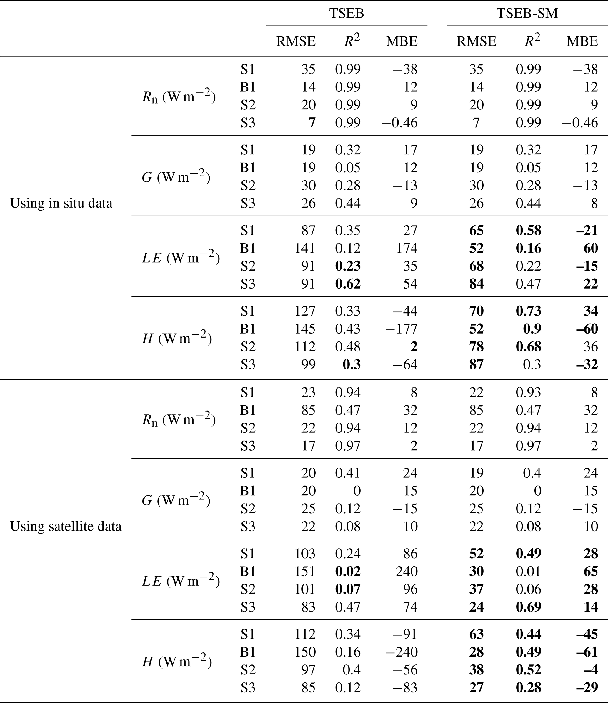
Table 4Statistical results (RMSE, R² and MBE) between modeled and measured sensible and latent heat fluxes for S1, S2, B1 and S3, and for TSEB and TSEB-SM models, separately (R_n and G are forced to their measured value). Bold values are the values with better statistical results.

Download Print Version | Download XLSX

For the S3 season, the error in daily retrieved α_PT at the beginning of the development stage has a strong impact on LE predictions and thus yields to greater discrepancies illustrated in Fig. 8. To overcome this error, the threshold on f_c to separate calibration steps 1 and 2 was increased to 0.63 (arbitrary value). The TSEB-SM model is then run using the new threshold. The LE simulations are improved, with a RMSE of 73 W m⁻² instead of 98 W m⁻² and a relative error (estimated as the RMSE divided by the mean observed LE) of about 42 % instead of 58 %. The increase in the threshold is intended to decrease the uncertainties in α_PT retrievals when vegetation is not fully covering the soil. It can be concluded that the errors in α_PT retrievals have a strong impact on LE estimates.

https://www.hydrol-earth-syst-sci.net/24/1781/2020/hess-24-1781-2020-f09

Figure 9Same as Fig. 8 but for H fluxes.

Download

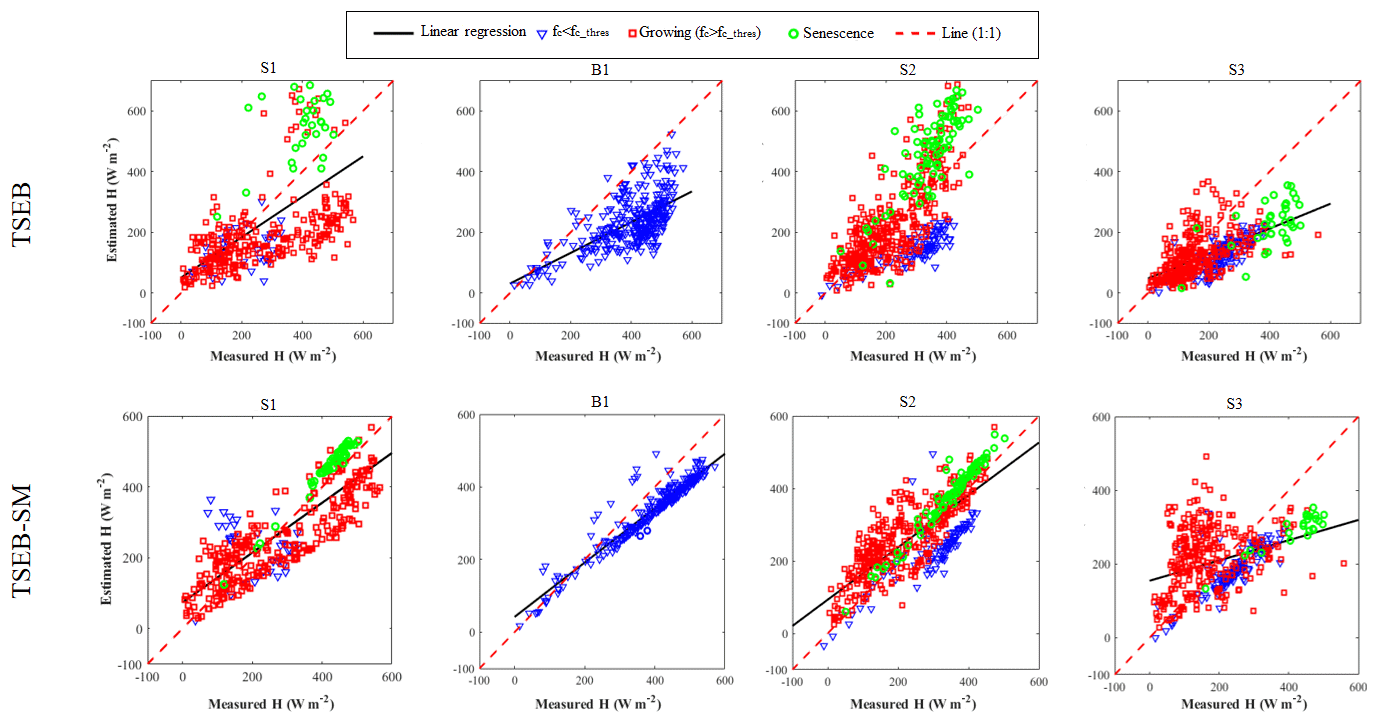
The ability of TSEB-SM to estimate the sensible heat fluxes is also investigated. Figure 9 displays the comparison between TSEB and TSEB-SM for each season and Table 4 summarizes the different statistical parameters. One can notice that TSEB shows greater discrepancies in H estimation, with a RMSE of about 127, 112 and 103 W m⁻² and a MBE of about −41, 1, and −71 W m⁻² for S1, S2 and S3, respectively. Both RMSE and MBE values are generally much reduced when using TSEB-SM, with RMSE values of about 68, 72, and 98 W m⁻² and MBE values of about −10, 24, and 7 W m⁻², respectively. During B1, TSEB model underestimates H. This can be explained by the low sensitivity of simulated sensible heat flux to changes in surface and atmospheric conditions, consistent with former results obtained on different sites of irrigated wheat (Ait Hssaine et al., 2018 b). The discrepancies between TSEB-SM and in situ H during S3 are mostly rectified by using the new threshold on f_c: the statistical results are improved, the RMSE is about 73 W m⁻² and the relative error is 39 % (instead of 52 %). It can be concluded that the uncertainty observed over the α_PT during the first few days of the development stage (25 January–4 March) is mainly related to the impact of the soil, which is not negligible during the first weeks of the growing stage. Nevertheless, by considering the overall results obtained for the three seasons, the threshold of $f_{c, thres} = 0.5$ can be considered an acceptable value to calibrate the soil resistance parameters and the Priestly–Taylor coefficient.

As a further step, the intercomparison between TSEB and TSEB-SM is evaluated by predicting R_n and G fluxes instead of forcing them to their measured values. The statistical results of the comparison between simulated and observed R_n, G, H and LE are listed in Table 5. The scattering obtained when comparing turbulent flux estimations to measurements is mainly related to the uncertainty in available energy estimates, mainly related to the uncertainty in soil heat flux estimates. Indeed, as reported in Table 5, R_n is very well simulated for both TSEB and TSEB-SM. The R² between simulated and observed R_n is about 0.99 during all seasons. Meanwhile, G shows a poor correlation, with an R² varying from 0.05 to 0.45. This is mainly linked to the approach used to estimate G, which requires local calibration. Kustas et al. (1998) hence indicated that the ratio $G / R_{n, soil}$ cannot be considered a constant, because it is affected by different factors such as time of day, moisture conditions and soil texture and structure.

https://www.hydrol-earth-syst-sci.net/24/1781/2020/hess-24-1781-2020-f10

Figure 10Same as Fig. 8 but for satellite data.

Download

https://www.hydrol-earth-syst-sci.net/24/1781/2020/hess-24-1781-2020-f11

Figure 11Same as Fig. 8 but for H fluxes and satellite data.

Download

https://www.hydrol-earth-syst-sci.net/24/1781/2020/hess-24-1781-2020-f12

Figure 12α_PT vs. residual H and LE error.

Download

3.3.2 Using satellite data

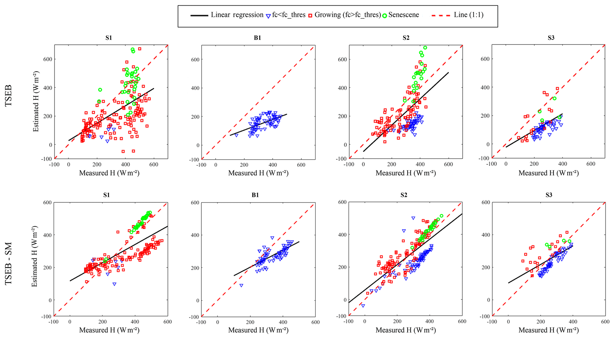
In order to gain greater insight into how TSEB and TSEB-SM models respond to different surface conditions across a landscape, an analysis of the spatial distributions and the magnitude of the turbulent fluxes using remotely sensing data produced from the two models is conducted. The comparisons between TSEB/TSEB-SM versus observed LE over the four seasons are illustrated in Fig. 10. Figure 10 indicates that TSEB overestimates latent heat flux. The overall MBE values are about 119, 181, 94 and 128 W m⁻² for S1, B1, S2 and S3, respectively. The overestimation of LE fluxes can be explained by the fact that α_PT is set to 1.26 during the entire agricultural season including stress conditions. This probably causes larger errors in the LE estimation, especially during the growing stage. Indeed, the saturation of TSEB during the senescence period is precisely caused by the PT coefficient fixed to 1.26. The errors are reduced when using TSEB-SM. In fact, the constraint on plant transpiration, while retrieving daily α_PT values improves ET estimates, especially for the growing stage. Moreover, during the senescence stage the large positive bias of LE is considerably reduced. In fact, the decrease in calibrated daily α_PT is associated with the drop in NDVI during senescence (Ait Hssaine et al., 2018 b). Additionally, the constraint on the soil evaporation via the DisPATCh SM clearly reduces the MBE values during the emergence period ( $f_{c} \leq f_{c, thres}$ ). Finally, the constraint applied on TSEB-SM output fluxes using LST-derived available energy and the TSEB-SM-derived evaporative fraction (Eq. 8) improves the LE estimates for the whole study period. The MBE values are about 39, 4, 7 and 62 W m⁻² for S1, S2, S3 and B1, respectively.

TSEB consistently exhibits larger errors in H estimation (see Fig. 11), with RMSE values up to 98, 73, 56 and 66 W m⁻² during S1, S2, S3 and B1, respectively. The RMSE is improved while using TSEB-SM, with values of about 55, 41, 24 and 27 W m⁻² during S1, S2, S3 and B1, respectively.

The intercomparison between TSEB and TSEB-SM is made by forcing the available energy to its measured value. The statistics listed in Table 5 indicate that there are similar differences between modeled versus measured R_n using either TSEB or TSEB-SM. Overall, the discrepancies between estimated and measured R_n are likely due to a greater scatter between MODIS and in situ measured LST. Note that RMSE values up to 6 K have been noted when comparing LST MODIS with ground-based measurements. These uncertainties are likely to be explained by the huge scale mismatch between the 1 km resolution of MODIS LST and the footprint size (approximately 1 m) of ground-based radiometers. The uncertainties in key input data generate large differences in simulated R_n compared to the tower measurements. The greater scatter between modeled and measured G from the two models reflects the fact that there is a major mismatch in scale between the area sampled by the soil heat flux sensors and the 1 km resolution of model inputs. It appears that the LE estimates from TSEB-SM are generally in closer agreement with the measurements than the TSEB model outputs. The RMSE is significantly improved from 103 to 52 W m⁻², from 151 to 30 W m², from 101 to 35 W m⁻² and from 83 to 24 W m⁻², during S1, B1, S2 and S3, respectively. For the sensible heat flux H, the difference between TSEB estimates and EC measurements listed in Table 5 indicates a fairly large underestimation, the MBE values varying between −56 and −240 W m⁻². However, the TSEB-SM output provides a quite significant improvement, with an absolute MBE lower than −61 W m⁻² during all seasons.

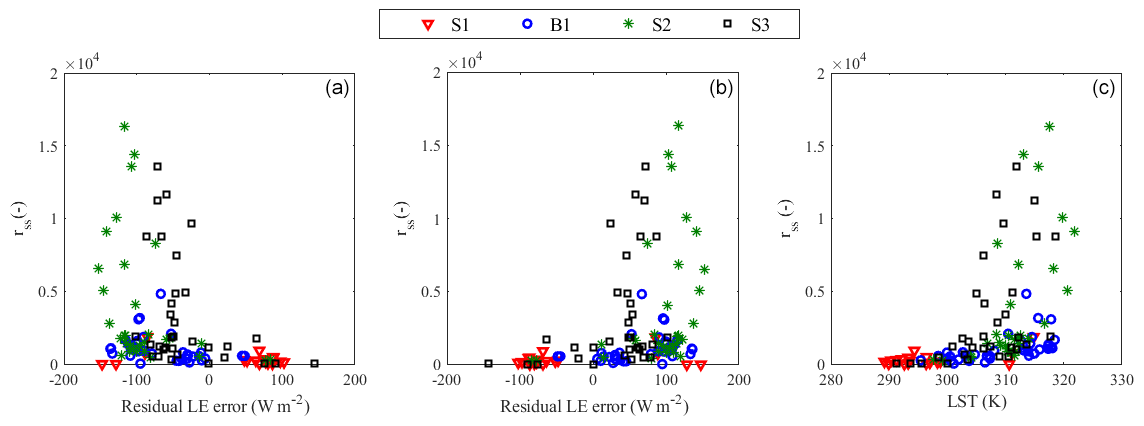
https://www.hydrol-earth-syst-sci.net/24/1781/2020/hess-24-1781-2020-f13

Figure 13Retrieved r_ss vs. residual H (a) and LE (b) error and LST (c) for the four study periods separately.

Download

https://www.hydrol-earth-syst-sci.net/24/1781/2020/hess-24-1781-2020-f14

Figure 14Residual H (a, c) and LE (b, d) errors vs. DisPATCh (a, b) and in situ (c, d) SM.

Download

Table 5Same as Table 2 but for simulated R_n and G. Bold values are the values with better statistical results.

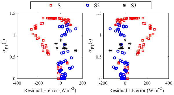
Download Print Version | Download XLSX

3.4 Evaluation of H and LE estimates

In this section, the residual error of the H and LE estimated with the TSEB-SM-retrieved soil/vegetation parameters is analyzed. Figure 12 plots retrieved α_PT vs. residual H and LE error. The retrieved α_PT is poorly correlated with residual H ( $R = - 0.27$ ) and ET (R=0.27) errors, especially for seasons S1 and S2. For season S3, few retrieved α_PT values were available because of the non-availability of MODIS products during cloudy days. It is shown that the trend between α_PT and residual H error is slightly negative for S1, while it is slightly positive for S2. According to these results, no information linked to the variability of α_PT versus residual ET and H errors can be derived. Figure 13 plots retrieved r_ss vs. residual H and LE error and LST for the four study periods. The retrieved r_ss is negatively correlated ( $R = - 0.33$ ) with residual H error (predicted–observed) for the four seasons, while it is positively correlated (R=0.33) with residual LE error. The residual error covers a wide range (between −150 and 150 W m⁻²) for the lower r_ss values, while it is biased for the higher r_ss values. Such a result indicates that the r_ss formulation as a function of near-surface SM needs further improvements (Merlin et al., 2016, 2018) in order to reduce systematic uncertainties in evaporation estimates, especially in dry (moisture-limited) conditions. Consistent with the general decrease in LST with SM, LST is positively correlated with retrieved r_ss (R=0.45). This is very coherent since r_ss decreases with the increase in SM. Regarding the sensitivity analysis of residual H and LE errors to observed SM, Fig. 14 shows that SM is positively correlated with residual H error, while it is negatively correlated with residual LE error for the entire study period. The correlation coefficient is about 0.3 when using DisPATCh SM, while it is about 0.4 when using in situ SM. This difference can be explained by the uncertainty (including spatial representativeness issues at the localized scale) in DisPATCh SM. The positive correlation coefficient between residual LE error and observed SM is likely to be due to the systematic errors in r_ss estimates for dry conditions as mentioned previously. For S2, B1 and S3, the residual H error ranges between −150 and 50 W m⁻² for SM between 0 and 0.10 m³ m⁻³, while it is slightly overestimated for the higher range of SM. The residual LE error is also found to be influenced by SM, but in the opposite sense.

4 Conclusions

The microwave-derived near-surface soil moisture (SM) from SMOS and the thermal-derived land surface temperature (LST) from MODIS are integrated simultaneously in the TSEB formalism within a calibration procedure to invert both the soil resistance to evaporation (constant parameters) and the PT coefficient based on a threshold on f_c. The TSEB-SM model is applied during a 4-year period (2014–2018) over a rainfed wheat field in the Tensift basin, central Morocco. Significant conclusions are given below.

The constraint applied on the soil evaporation represented explicitly as a function of SM via a soil resistance term reduces the errors when using TSEB-SM instead of TSEB.

The first step of the TSEB-SM approach is to calibrate r_ss for ( $f_{c} \leq f_{c, thres}$ ) at Terra and Aqua overpass times. Despite the scale difference between the MODIS/DisPATCh resolution data and the footprint size of in situ measurements, the parameters (a_rss, b_rss) calculated for the entire study period using satellite data are relatively close to those derived from in situ measurements.
The second step of the TSEB-SM approach is to invert the α_PT on a daily basis for $f_{c} > f_{c, thres}$ by using LST and SM data. The maximum values of daily calibrated α_PT are 1.38, 1.25 and 0.87, when using satellite data, for S1, S2 and S3, respectively. Those values are in accordance with the total rainfall amounts, which were about 608, 214 and 421 mm per wheat season for S1, S2 and S3, respectively. S1 and S2 have the same distribution of daily calibrated α_PT when compared with the α_PT retrieved using in situ data, while the retrieved α_PT remains at a mostly constant value (∼0.7) throughout the S3 study period because of the non-availability of MODIS products during cloudy days.
Finally, an analysis of the spatial distributions and the magnitude of the turbulent fluxes using remotely sensing data produced from the two models were conducted. TSEB exhibits larger errors in H and LE estimates. These uncertainties can be linked to the theoretical value of α_PT, which is fixed to 1.26 for the whole study period as well as to the scale mismatch between the 1 km resolution of MODIS LST and the footprint size (approximately 1 m) of the ground-based radiometer.

As a short-term prospect, the use of high-resolution products from active sensors (Sentinel-1) would allow application of the TSEB-SM approach at the field scale over heterogeneous (e.g., irrigated) landscapes. Also, the robustness of TSEB-SM in terms of evaporation/transpiration partitioning will be tested by using independent flux measurements derived from lysimeters and sap flow sensors (Rafi et al., 2019). In addition, the evaluation of ET at large scale is missing. Spatialized measurements that could be collected by scintillometers installed at various points in the region would be a solution for that purpose.

Data availability

The data that support the findings of this study are available from the authors, but restrictions apply to the availability of these data, which were carried out within the framework of several projects and so are not publicly available. Data are however available from the authors upon reasonable request and with permission of the co-directors of the LMI TREMA laboratory.

Author contributions

BAH and OM developed the idea of the study, designed the methodology of the work, verified/discussed the results and wrote the original draft of the manuscript. BAH analyzed the data and validated the results. BAH, OM, and JE investigated the experimental protocol and contributed to materials/analysis tools. BAH and NO contributed to remote sensing data processing. OM and SK supervised the work. BAH, OM, JE, SK, and SE contributed to the final manuscript.

Competing interests

The authors declare that they have no conflict of interest.

Acknowledgements

The study was carried out in the framework of the Joint International Laboratory TREMA https://www.lmi-trema.ma (last access: 4 April 2020), and funded by the European Commission Horizon 2020 Programme for Research and Innovation (H2020) in the context of the Marie Sklodowska-Curie Research and Innovation Staff Exchange (RISE) action (REC project, grant agreement no: 645642), followed by ACCWA project, grant agreement no. 823965). Additional funding was provided by the ERANETMED03-62 CHAAMS, the French Agence Nationale de la Recherche (MIXMOD-E project. ANR-13-JS06-003-01) and PHC TBK/18/61 projects. We deeply grateful to the ARTS fellowship program from Institut de Recherche pour le Développement (IRD) for awarding a PhD scholarship to Bouchra Ait Hssaine.

Review statement

This paper was edited by Bob Su and reviewed by Xuelong Chen and two anonymous referees.

References

Agam, N., Kustas, W. P., Anderson, M. C., Norman, J. M., Colaizzi, P. D., Howell, T. A., Prueger, J. H., Meyers, T. P., and Wilson, T. B.: Application of the Priestley–Taylor Approach in a Two-Source Surface Energy Balance Model, J. Hydrometeorol., 11, 185–198, https://doi.org/10.1175/2009JHM1124.1, 2010. a

Ait Hssaine, B., Ezzahar, J., Jarlan, L., Merlin, O., Khabba, S., Brut, A., Er-Raki, S., Elfarkh, J., Cappelaere, B., and Chehbouni, G.: Combining a Two Source Energy Balance Model Driven by MODIS and MSG-SEVIRI Products with an Aggregation Approach to Estimate Turbulent Fluxes over Sparse and Heterogeneous Vegetation in Sahel Region (Niger), Remote Sens., 10, 974, https://doi.org/10.3390/rs10060974, 2018a. a, b

Ait Hssaine, B., Merlin, O., Rafi, Z., Ezzahar, J., Jarlan, L., Khabba, S., and Er-Raki, S.: Calibrating an evapotranspiration model using radiometric surface temperature, vegetation cover fraction and near-surface soil moisture data, Agr. Forest Meteorol., 256–257, 104–115, https://doi.org/10.1016/j.agrformet.2018.02.033, 2018b. a, b, c, d, e, f, g, h, i, j, k, l

Ali Eweys, O., José Escorihuela, M., Villar, J. M., Er-Raki, S., Amazirh, A., Olivera, L., Jarlan, L., Khabba, S., and Merlin, O.: Remote sensing Disaggregation of SMOS Soil Moisture to 100 m Resolution Using MODIS Optical/Thermal and Sentinel-1 Radar Data: Evaluation over a Bare Soil Site in Morocco, Remote Sens., 9, 1155, https://doi.org/10.3390/rs9111155, 2017. a

Allen, R. G., Pereira, L. S., Raes, D., and Smith, M.: Crop evapotranspiration – Guidelines for computing crop water requirements, FAO Irrigation and drainage paper 56, Tech. rep., available at: https://appgeodb.nancy.inra.fr/biljou/pdf/Allen_FAO1998.pdf (last access: 4 April 2020), 1998. a, b

Amazirh, A., Er-Raki, S., Chehbouni, A., Rivalland, V., Diarra, A., Khabba, S., Ezzahar, J., and Merlin, O.: Modified Penman–Monteith equation for monitoring evapotranspiration of wheat crop: Relationship between the surface resistance and remotely sensed stress index, Biosyst. Eng., 164, 68–84, https://doi.org/10.1016/j.biosystemseng.2017.09.015, 2017. a

Amazirh, A., Merlin, O., Er-Raki, S., Gao, Q., Rivalland, V., Malbeteau, Y., Khabba, S., and Escorihuela, M. J.: Retrieving surface soil moisture at high spatio-temporal resolution from a synergy between Sentinel-1 radar and Landsat thermal data: A study case over bare soil, Remote Sens. Environ., 211, 321–337, https://doi.org/10.1016/j.rse.2018.04.013, 2018. a

Anderson, M. C., Norman, J. M., Mecikalski, J. R., Otkin, J. A., and Kustas, W. P.: A climatological study of evapotranspiration and moisture stress across the continental United States based on thermal remote sensing: 2. Surface moisture climatology, J. Geophys. Res., 112, D11112, https://doi.org/10.1029/2006JD007507, 2007. a

Bandara, R., Walker, J. P., Rüdiger, C., and Merlin, O.: Towards soil property retrieval from space: An application with disaggregated satellite observations, J. Hydrol., 522, 582–593, https://doi.org/10.1016/j.jhydrol.2015.01.018, 2015. a

Bastiaanssen, W. G. and Ali, S.: A new crop yield forecasting model based on satellite measurements applied across the Indus Basin, Pakistan, Agr. Ecosyst. Environ., 94, 321–340, https://doi.org/10.1016/S0167-8809(02)00034-8, 2003. a

Bhattarai, N., Mallick, K., Stuart, J., Vishwakarma, B. D., Niraula, R., Sen, S., and Jain, M.: An automated multi-model evapotranspiration mapping framework using remotely sensed and reanalysis data, Remote Sens. Environ., 229, 69–92, https://doi.org/10.1016/j.rse.2019.04.026, 2019. a

Bindlish, R., Kustas, W. P., French, A. N., Diak, G. R., and Mecikalski, J. R.: Influence of near-surface soil moisture on regional scale heat fluxes: Model results using microwave remote sensing data from SGP97, IEEE T. Geosci. Remote, 39, 1719–1728, https://doi.org/10.1109/36.942550, 2001. a, b

Boulet, G., Mougenot, B., Lhomme, J. P., Fanise, P., Lili-Chabaane, Z., Olioso, A., Bahir, M., Rivalland, V., Jarlan, L., Merlin, O., Coudert, B., Er-Raki, S., and Lagouarde, J. P.: The SPARSE model for the prediction of water stress and evapotranspiration components from thermal infra-red data and its evaluation over irrigated and rainfed wheat, Hydrol. Earth Syst. Sci., 19, 4653–4672, https://doi.org/10.5194/hess-19-4653-2015, 2015. a, b, c

Brutsaert, W.: Introduction, in: Evaporation into the Atmosphere, Springer Netherlands, Dordrecht, 1–11, https://doi.org/10.1007/978-94-017-1497-6_1, 1982. a

Chanzy, A. and Bruckler, L.: Significance of soil surface moisture with respect to daily bare soil evaporation, Water Resour. Res., 29, 1113–1125, https://doi.org/10.1029/92WR02747, 1993. a

Chirouze, J., Boulet, G., Jarlan, L., Fieuzal, R., Rodriguez, J. C., Ezzahar, J., Bigeard, G., and Merlin, O.: Intercomparison of four remote-sensing-based energy balance methods to retrieve surface evapotranspiration and water stress of irrigated fields in semi-arid climate, Hydrol. Earth Syst. Sci., 18, 1165–1188, https://doi.org/10.5194/hess-18-1165-2014, 2014. a, b

Choudhury, B., Idso, S., and Reginato, R.: Analysis of an empirical model for soil heat flux under a growing wheat crop for estimating evaporation by an infrared-temperature based energy balance equation, Agr. Forest Meteorol., 39, 283–297, https://doi.org/10.1016/0168-1923(87)90021-9, 1987. a

Colaizzi, P. D., Kustas, W. P., Anderson, M. C., Agam, N., Tolk, J. A., Evett, S. R., Howell, T. A., Gowda, P. H., and O'shaughnessy, S. A.: Two-source energy balance model estimates of evapotranspiration using component and composite surface temperatures q, Adv. Water Resour., 50, 134–151, https://doi.org/10.1016/j.advwatres.2012.06.004, 2012. a

Colliander, A., Fisher, J. B., Halverson, G., Merlin, O., Misra, S., Bindlish, R., Jackson, T. J., and Yueh, S.: Spatial Downscaling of SMAP Soil Moisture Using MODIS Land Surface Temperature and NDVI during SMAPVEX15, IEEE Geosci. Remote Sens. Lett., 14, 2107–2111, https://doi.org/10.1109/LGRS.2017.2753203, 2017. a

Cosby, B. J., Hornberger, G. M., Clapp, R. B., and Ginn, T. R.: A Statistical Exploration of the Relationships of Soil Moisture Characteristics to the Physical Properties of Soils, Tech. Rep. 6, available at: http://denning.atmos.colostate.edu/readings/Land/Water_Resour._Res._1984_Cosby.pdf (last access: 4 April 2020), 1984. a

Djamai, N., Magagi, R., Goita, K., Merlin, O., Kerr, Y., and Walker, A.: Disaggregation of SMOS soil moisture over the Canadian Prairies, Remote Sens. Environ., 170, 255–268, https://doi.org/10.1016/j.rse.2015.09.013, 2015. a

Entekhabi, D., Njoku, E. G., O'Neill, P. E., Kellogg, K. H., Crow, W. T., Edelstein, W. N., Entin, J. K., Goodman, S. D., Jackson, T. J., Johnson, J., Kimball, J., Piepmeier, J. R., Koster, R. D., Martin, N., McDonald, K. C., Moghaddam, M., Moran, S., Reichle, R., Shi, J. C., Spencer, M. W., Thurman, S. W., Tsang, L., and Van Zyl, J.: The Soil Moisture Active Passive (SMAP) Mission, Proc. IEEE, 98, 704–716, https://doi.org/10.1117/12.795910, 2010. a

Er-Raki, S., Chehbouni, A., Guemouria, N., Duchemin, B., Ezzahar, J., and Hadria, R.: Combining FAO-56 model and ground-based remote sensing to estimate water consumptions of wheat crops in a semi-arid region, Agr. Water Manage., 87, 41–54, https://doi.org/10.1016/j.agwat.2006.02.004, 2007. a

Escorihuela, M. J. and Quintana-Seguí, P.: Comparison of remote sensing and simulated soil moisture datasets in Mediterranean landscapes, Remote Sens. Environ., 180, 99–114, https://doi.org/10.1016/j.rse.2016.02.046, 2016. a

Escorihuela, M. J., Chanzy, A., Wigneron, J., and Kerr, Y.: Effective soil moisture sampling depth of L-band radiometry: A case study, Remote Sens. Environ., 114, 995–1001, https://doi.org/10.1016/J.RSE.2009.12.011, 2010. a

Escorihuela, M. J., Merlin, O., Stefan, V., Moyano, G., Eweys, O. A., Zribi, M., Kamara, S., Benahi, A. S., Abdallahi, M., Ebbe, B., Chihrane, J., Ghaout, S., Cissé, S., Diakité, F., Lazar, M., Pellarin, T., Grippa, M., Cressman, K., and Piou, C.: SMOS based high resolution soil moisture estimates for desert locust preventive management, Remote Sens. Appl.: Soc. Environ., 11, 140–150, https://doi.org/10.1016/j.rsase.2018.06.002, 2018. a

Fisher, J. B., Tu, K. P., and Baldocchi, D. D.: Global estimates of the land-atmosphere water flux based on monthly AVHRR and ISLSCP-II data, validated at 16 FLUXNET sites, Remote Sens. Environ., 112, 901–919, https://doi.org/10.1016/j.rse.2007.06.025, 2008. a, b

Fisher, J. B., Melton, F., Middleton, E., Hain, C., Anderson, M., Allen, R., Mccabe, M. F., Hook, S., Baldocchi, D., Townsend, P. A., Kilic, A., Tu, K., Miralles, D. D., Perret, J., Lagouarde, J.-P., Waliser, D., Purdy, A. J., French, A., Schimel, D., Famiglietti, J. S., Stephens, G., and Wood, E. F.: The future of evapotranspiration: Global requirements for ecosystem functioning, carbon and climate feedbacks, agricultural management, and water resources, Water Resour. Res., 53,, 2618–2626, https://doi.org/10.1002/2016WR020175, 2017. a

Gan, G. and Gao, Y.: Estimating time series of land surface energy fluxes using optimized two source energy balance schemes: Model formulation, calibration, and validation, Agr. Forest Meteorol., 208, 62–75, https://doi.org/10.1016/j.agrformet.2015.04.007, 2015. a

Gentine, P., Entekhabi, D., Polcher, J., Gentine, P., Entekhabi, D., and Polcher, J.: The Diurnal Behavior of Evaporative Fraction in the Soil–Vegetation–Atmospheric Boundary Layer Continuum, J. Hydrometeorol., 12, 1530–1546, https://doi.org/10.1175/2011JHM1261.1, 2011. a

Gerhards, M., Schlerf, M., Mallick, K., and Udelhoven, T.: Challenges and future perspectives of multi-/Hyperspectral thermal infrared remote sensing for crop water-stress detection: A review, Remote Sens., 11, 1240, https://doi.org/10.3390/rs11101240, 2019. a

Gokmen, M., Vekerdy, Z., Verhoef, A., Verhoef, W., Batelaan, O., and Tol, C. V. D.: Remote Sensing of Environment Integration of soil moisture in SEBS for improving evapotranspiration estimation under water stress conditions, Remote Sens. Environ., 121, 261–274, https://doi.org/10.1016/j.rse.2012.02.003, 2012. a, b

Gonzalez-dugo, M. P., Neale, C. M. U., Mateos, L., Kustas, W. P., Prueger, J. H., Anderson, M. C., and Li, F.: Agricultural and Forest Meteorology A comparison of operational remote sensing-based models for estimating crop evapotranspiration, Agr. Forest Meteorol., 149, 1843–1853, https://doi.org/10.1016/j.agrformet.2009.06.012, 2009. a

Jarlan, L., Khabba, S., Er-Raki, S., Le Page, M., Hanich, L., Fakir, Y., Merlin, O., Mangiarotti, S., Gascoin, S., Ezzahar, J., Kharrou, M. H., Berjamy, B., Saaïdi, A., Boudhar, A., Benkaddour, A., Laftouhi, N., Abaoui, J., Tavernier, A., Boulet, G., Simonneaux, V., Driouech, F., El Adnani, M., El Fazziki, A., Amenzou, N., Raibi, F., El Mandour, A., Ibouh, H., Le Dantec, V., Habets, F., Tramblay, Y., Mougenot, B., Leblanc, M., El Faïz, M., Drapeau, L., Coudert, B., Hagolle, O., Filali, N., Belaqziz, S., Marchane, A., Szczypta, C., Toumi, J., Diarra, A., Aouade, G., Hajhouji, Y., Nassah, H., Bigeard, G., Chirouze, J., Boukhari, K., Abourida, A., Richard, B., Fanise, P., Kasbani, M., Chakir, A., Zribi, M., Marah, H., Naimi, A., Mokssit, A., Kerr, Y., and Escadafal, R.: Remote Sensing of Water Resources in Semi-Arid Mediterranean Areas: the joint international laboratory TREMA, Int. J. Remote Sens., 36, 4879–4917, https://doi.org/10.1080/01431161.2015.1093198, 2015. a

Jin, Y., Randerson, J. T., and Goulden, M. L.: Continental-scale net radiation and evapotranspiration estimated using MODIS satellite observations, Remote Sens. Environ., 115, 2302–2319, https://doi.org/10.1016/j.rse.2011.04.031, 2011. a

Kerr, Y. H., Waldteufel, P., Wigneron, J.-P., Delwart, S., Cabot, F., Boutin, J., Escorihuela, M.-J., Font, J., Reul, N., Gruhier, C., Juglea, S. E., Drinkwater, M. R., Hahne, A., Martín-Neira, M., Mecklenburg, S., Kerr, Y. H., Cabot, F., Gruhier, C., Juglea, S. E., Wigneron, J.-P., Delwart, S., Drinkwater, M. R., Hahne, A., and Martín, M.: The SMOS Mission: New Tool for Monitoring Key Elements of the Global Water Cycle, Proc. IEEE, 98, 666–687, https://doi.org/10.1109/JPROC.2010.2043032, 2010. a

Kerr, Y. H., Member, S., Waldteufel, P., Richaume, P., Pierre Wigneron, J., Ferrazzoli, P., Mahmoodi, A., Al Bitar, A., Cabot, F., Gruhier, C., Enache Juglea, S., Leroux, D., Mialon, A., Delwart, S., Kerr, Y. H., Richaume, P., Al Bitar, A., Cabot, F., Gruhier, C., Juglea, S. E., Leroux, D., Mialon, A., and Wigneron, J. P.: The SMOS Soil Moisture Retrieval Algorithm, IEEE T. Geosci. Remote, 50, 1384–1403, https://doi.org/10.1109/TGRS.2012.2184548, 2012. a

Kharrou, M. H., Er-Raki, S., Chehbouni, A., Duchemin, B., Simonneaux, V., Lepage, M., Ouzine, L., and Jarlan, L.: Water use efficiency and yield of winter wheat under different irrigation regimes in a semi-arid region, Agricult. Sci., 2, 273–282, https://doi.org/10.4236/as.2011.23036, 2011. a

Kustas, W. P. and Norman, J. M.: A two-source approach for estimating turbulent fluxes using multiple angle thermal infrared observations, Water Resour. Res., 33, 1495–1508, https://doi.org/10.1029/97WR00704, 1997. a

Kustas, W. P. and Norman, J.: Evaluation of soil and vegetation heat flux predictions using a simple two-source model with radiometric temperatures for partial canopy cover, Agr. Forest Meteorol., 94, 13–29, https://doi.org/10.1016/S0168-1923(99)00005-2, 1999. a

Kustas, W. P., Zhan, X., and Schmugge, T. J.: Combining optical and microwave remote sensing for mapping energy fluxes in a semiarid watershed, Remote Sens. Environ., 64, 116–131, https://doi.org/10.1016/S0034-4257(97)00176-4, 1998. a, b, c

Kustas, W. P., Zhan, X., and Jackson, T.: Mapping surface energy flux partitioning at large scales with optical and microwave remote sensing data from Washita '92, Water Resour. Res., 35, 265–277, https://doi.org/10.1029/98WR02094, 1999. a, b

Lewis, P. and Barnsley, M. J.: Influence of the sky radiance distribution on various formulations of the earth surface albedo, Remote Sensing Unit, 707–715, available at: http://www2.geog.ucl.ac.uk/~plewis/LewisBarnsley1994.pdf (last access: 4 April 2020), 1994. a

Lhomme, J.-P. and Elguero, E.: Examination of evaporative fraction diurnal behaviour using a soil-vegetation model coupled with a mixed-layer model, Hydrol. Earth Syst. Sci., 3, 259–270, https://doi.org/10.5194/hess-3-259-1999, 1999. a

Li, F., Kustas, W. P., Anderson, M. C., Jackson, T. J., Bindlish, R., and Prueger, J. H.: Comparing the utility of microwave and thermal remote-sensing constraints in two-source energy balance modeling over an agricultural landscape, Remote Sens. Environ., 101, 315–328, https://doi.org/10.1016/j.rse.2006.01.001, 2006. a, b, c, d, e, f

Lievens, H., Tomer, S. K., Al Bitar, A., De Lannoy, G. J., Drusch, M., Dumedah, G., Hendricks Franssen, H. J., Kerr, Y. H., Martens, B., Pan, M., Roundy, J. K., Vereecken, H., Walker, J. P., Wood, E. F., Verhoest, N. E., and Pauwels, V. R.: SMOS soil moisture assimilation for improved hydrologic simulation in the Murray Darling Basin, Australia, Remote Sens. Environ., 168, 146–162, https://doi.org/10.1016/j.rse.2015.06.025, 2015. a

Littell, J. S., Peterson, D. L., Riley, K. L., Liu, Y., and Luce, C. H.: A review of the relationships between drought and forest fire in the United States, Global Change Biol., 22, 2353–2369, https://doi.org/10.1111/gcb.13275, 2016. a

Long, D. and Singh, V. P.: A Two-source Trapezoid Model for Evapotranspiration (TTME) from satellite imagery, Remote Sens. Environ., 121, 370–388, https://doi.org/10.1016/j.rse.2012.02.015, 2012. a

Madugundu, R., Al-Gaadi, K. A., Tola, E., Hassaballa, A. A., and Patil, V. C.: Performance of the METRIC model in estimating evapotranspiration fluxes over an irrigated field in Saudi Arabia using Landsat-8 images, Hydrol. Earth Syst. Sci., 21, 6135–6151, https://doi.org/10.5194/hess-21-6135-2017, 2017. a

Malbéteau, Y., Merlin, O., Molero, B., Rüdiger, C., and Bacon, S.: DisPATCh as a tool to evaluate coarse-scale remotely sensed soil moisture using localized in situ measurements: Application to SMOS and AMSR-E data in Southeastern Australia, Int. J. Appl. Earth Observ. Geoinform., 45, 221–234, https://doi.org/10.1016/j.jag.2015.10.002, 2016. a, b, c, d, e

Malbéteau, Y., Merlin, O., Balsamo, G., Er-Raki, S., Khabba, S., Walker, J. P., and Jarlan, L.: Toward a Surface Soil Moisture Product at High Spatiotemporal Resolution: Temporally Interpolated, Spatially Disaggregated SMOS Data, J. Hydrometeorol., 19, 183–200, https://doi.org/10.1175/JHM-D-16-0280.1, 2018. a, b

Mallick, K., Jarvis, A. J., Boegh, E., Fisher, J. B., Drewry, D. T., Tu, K. P., Hook, S. J., Hulley, G., Ardö, J., Beringer, J., Arain, A., and Niyogi, D.: A Surface Temperature Initiated Closure (STIC) for surface energy balance fluxes, Remote Sens. Environ., 141, 243–261, https://doi.org/10.1016/j.rse.2013.10.022, 2014. a

Mallick, K., Boegh, E., Trebs, I., Alfieri, J. G., Kustas, W. P., Prueger, J. H., Niyogi, D., Das, N., Drewry, D. T., Hoffmann, L., and Jarvis, A. J.: Penman–Monteith formulation, Water Resour. Res., 51, 6214–6243, https://doi.org/10.1002/2014WR016106, 2015. a

Mallick, K., Trebs, I., Boegh, E., Giustarini, L., Schlerf, M., Drewry, D. T., Hoffmann, L., Von Randow, C., Kruijt, B., Araùjo, A., Saleska, S., Ehleringer, J. R., Domingues, T. F., Ometto, J. P. H., Nobre, A. D., Luiz Leal De Moraes, O., Hayek, M., William Munger, J., and Wofsy, S. C.: Canopy-scale biophysical controls of transpiration and evaporation in the Amazon Basin, Hydrol. Earth Syst. Sci., 20, 4237–4264, https://doi.org/10.5194/hess-20-4237-2016, 2016. a

Mallick, K., Toivonen, E., Trebs, I., Boegh, E., Cleverly, J., Eamus, D., Koivusalo, H., Drewry, D., Arndt, S. K., Griebel, A., Beringer, J., and Garcia, M.: Bridging Thermal Infrared Sensing and Physically-Based Evapotranspiration Modeling: From Theoretical Implementation to Validation Across an Aridity Gradient in Australian Ecosystems, Water Resour. Res., 54, 3409–3435, https://doi.org/10.1029/2017WR021357, 2018. a, b

Merlin, O., Al Bitar, A., Rivalland, V., Béziat, P., Ceschia, E., and Dedieu, G.: An analytical model of evaporation efficiency for unsaturated soil surfaces with an arbitrary thickness, J. Appl. Meteorol. Clim., 50, 457–471, https://doi.org/10.1175/2010JAMC2418.1, 2011. a, b

Merlin, O., Rüdiger, C., Al Bitar, A., Richaume, P., Walker, J. P., and Kerr, Y. H.: Disaggregation of SMOS soil moisture in Southeastern Australia, IEEE T. Geosci. Remote, 50, 1556–1571, https://doi.org/10.1109/TGRS.2011.2175000, 2012. a, b

Merlin, O., Escorihuela, M. J., Mayoral, M. A., Hagolle, O., Al Bitar, A., and Kerr, Y.: Self-calibrated evaporation-based disaggregation of SMOS soil moisture: An evaluation study at 3 km and 100 m resolution in Catalunya, Spain, Remote Sens. Environ., 130, 25–38, https://doi.org/10.1016/j.rse.2012.11.008, 2013. a, b, c, d

Merlin, O., Malbéteau, Y., Notfi, Y., Bacon, S., Er-Raki, S., Khabba, S., and Jarlan, L.: Performance metrics for soil moisture downscaling methods: Application to DISPATCH data in central Morocco, Remote Sens., 7, 3783–3807, https://doi.org/10.3390/rs70403783, 2015. a

Merlin, O., Stefan, V. G., Amazirh, A., Chanzy, A., Ceschia, E., Tallec, T., Beringer, J., Gentine, P., Er-Raki, S., Bircher, S., and Khabba, S.: Modeling soil evaporation efficiency in a range of soil and atmospheric conditions: A downward approach based on multi-site data, Water Resour. Res., 52, 3663–3684, https://doi.org/10.1002/2015WR018233, 2016. a, b, c

Merlin, O., Olivera-Guerra, L., Aït Hssaine, B., Amazirh, A., Rafi, Z., Ezzahar, J., Gentine, P., Khabba, S., Gascoin, S., and Er-Raki, S.: A phenomenological model of soil evaporative efficiency using surface soil moisture and temperature data, Agr. Forest Meteorol., 256–257, 501–515, https://doi.org/10.1016/J.AGRFORMET.2018.04.010, 2018. a, b, c, d, e

Molden, D., Oweis, T., Steduto, P., Bindraban, P., Hanjra, M. A., and Kijne, J.: Improving agricultural water productivity: Between optimism and caution, Agr. Water Manage., 97, 528–535, https://doi.org/10.1016/J.AGWAT.2009.03.023, 2010. a

Molero, B., Merlin, O., Malbéteau, Y., Al Bitar, A., Cabot, F., Stefan, V., Kerr, Y., Bacon, S., Cosh, M., Bindlish, R., and Jackson, T.: SMOS disaggregated soil moisture product at 1 km resolution: Processor overview and first validation results, Remote Sens. Environ., 180, 361–376, https://doi.org/10.1016/J.RSE.2016.02.045, 2016. a, b, c

Moran, M. S., Clarke, T. R., Inoue, Y., and Vidal, A.: Estimating Crop Water Deficit Using the Relation between Surface-Air Temperature and Spectral Vegetation Index, Remote Sens. Environ., 49, 246–263, 1994. a, b

Morillas, L., Villagarcía, L., Domingo, F., Nieto, H., Uclés, O., and García, M.: Environmental factors affecting the accuracy of surface fluxes from a two-source model in Mediterranean drylands: Upscaling instantaneous to daytime estimates, Agr. Forest Meteorol., 189–190, 140–158, https://doi.org/10.1016/j.agrformet.2014.01.018, 2014. a

Njoku, E. G., Jackson, T. J., Lakshmi, V., Member, S., Chan, T. K., and Nghiem, S. V.: Soil Moisture Retrieval From AMSR-E, IEEE T. Geosci. Remote, 41, 215–229, https://doi.org/10.1109/TGRS.2002.808243, 2003. a

Norman, J. M., Kustas, W. P., and Humes, K. S.: Source approach for estimating soil and vegetation energy fluxes in observations of directional radiometric surface temperature, Agr. Forest Meteorol., 77, 263–293, https://doi.org/10.1016/0168-1923(95)02265-Y, 1995. a, b, c, d

Ojha, N., Merlin, O., Molero, B., Suere, C., Olivera-Guerra, L., Ait Hssaine, B., Amazirh, A., Al Bitar, A., Escorihuela, M., and Er-Raki, S.: Stepwise Disaggregation of SMAP Soil Moisture at 100 m Resolution Using Landsat-7/8 Data and a Varying Intermediate Resolution, Remote Sens., 11, 1863, https://doi.org/10.3390/rs11161863, 2019. a

Olivera-Guerra, L., Merlin, O., Er-Raki, S., Khabba, S., and Escorihuela, M. J.: Estimating the water budget components of irrigated crops: Combining the FAO-56 dual crop coefficient with surface temperature and vegetation index data, Agr. Water Manage., 208, 120–131, https://doi.org/10.1016/j.agwat.2018.06.014, 2018. a

Owe, M., De Jeu, R., and Holmes, T.: Multisensor historical climatology of satellite-derived global land surface moisture, J. Geophys. Res., 113, 1002, https://doi.org/10.1029/2007JF000769, 2008. a

Peng, J., Loew, A., Merlin, O., and Verhoest, N. E.: A review of spatial downscaling of satellite remotely sensed soil moisture, Rev. Geophys., 55, 341–366, https://doi.org/10.1002/2016RG000543, 2017. a, b

Priestley, C. H. B. and Taylor, R. J.: On the Assessment of Surface Heat Flux and Evaporation Using Large-Scale Parameters, Mon. Weather Rev., 100, 81–92, https://doi.org/10.1175/1520-0493(1972)100<0081:OTAOSH>2.3.CO;2, 1972. a

Rafi, Z., Merlin, O., Le Dantec, V., Khabba, S., Mordelet, P., Er-Raki, S., Amazirh, A., Olivera-Guerra, L., Ait Hssaine, B., Simonneaux, V., Ezzahar, J., and Ferrer, F.: Partitioning evapotranspiration of a drip-irrigated wheat crop: Inter-comparing eddy covariance-, sap flow-, lysimeter- and FAO-based methods, Agr. Forest Meteorol., 265, 310–326, https://doi.org/10.1016/J.agrformet.2018.11.031, 2019. a

Roerink, G., Su, Z., and Menenti, M.: S-SEBI: A simple remote sensing algorithm to estimate the surface energy balance, Phys. Chem. Earth Pt. B, 25, 147–157, https://doi.org/10.1016/S1464-1909(99)00128-8, 2000. a

Sabaghy, S., Walker, J. P., Renzullo, L. J., Akbar, R., Chan, S., Chaubell, J., Das, N., Dunbar, R. S., Entekhabi, D., Gevaert, A., Jackson, T. J., Loew, A., Merlin, O., Moghaddam, M., Peng, J., Peng, J., Piepmeier, J., Rüdiger, C., Stefan, V., Wu, X., Ye, N., and Yueh, S.: Comprehensive analysis of alternative downscaled soil moisture products, Remote Sens. Environ., 239, 111586, https://doi.org/10.1016/j.rse.2019.111586, 2020. a

Sauer, T., Norman, J., Tanner, C., and Wilson, T.: Measurement of heat and vapor transfer coefficients at the soil surface beneath a maize canopy using source plates, Agr. Forest Meteorol., 75, 161–189, https://doi.org/10.1016/0168-1923(94)02209-3, 1995. a

Schmid, H. P.: Source areas for scalars and scalar fluxes, Bound.-Lay. Meteorol., 67, 293–318, https://doi.org/10.1007/BF00713146, 1994. a

Sellers, P. J., Heiser, M. D., and Hall, F. G.: Relations between surface conductance and spectral vegetation indexes at intermediate (100 m² to 15 km²) length scales, J. Geophys. Res.-Atmos., 97, 19033–19059, 1992. a, b, c, d, e

Shuttleworth, W., Gurney, R., Hsu, A., and Ormsby, J.: FIFE: the variation in energy partition at surface flux sites, Remote Sensing and Large-Scale Global Porcesses (IAHS Publ.), 186, 67–74, 1989. a

Su, Z.: The Surface Energy Balance System (SEBS) for estimation of turbulent heat fluxes, Hydrol. Earth Syst. Sci., 6, 85–100, https://doi.org/10.5194/hess-6-85-2002, 2002. a

Tasumi, M.: Estimating evapotranspiration using METRIC model and Landsat data for better understandings of regional hydrology in the western Urmia Lake Basin, Agr. Water Manage., 226, 105805, https://doi.org/10.1016/j.agwat.2019.105805, 2019. a

Twine, T. E., Kustas, W. P., Norman, J. M., Cook, D. R., Houser, P. R., Meyers, T. P., Prueger, J. H., Starks, P. J., Wesley, M. L., and Wesely, M. L.: Correcting eddy-covariance flux underestimates over a grassland, Tech. rep., available at: https://digitalcommons.unl.edu/cgi/viewcontent.cgi?article=1010&context=nasapub (last access: 4 April 2020), 2000. a

Wang, Y., Li, X., and Tang, S.: Validation of the SEBS-derived sensible heat for FY3A/VIRR and TERRA/MODIS over an alpine grass region using LAS measurements, Int. J. Appl. Earth Obs. Geoinform., 23, 226–233, https://doi.org/10.1016/j.jag.2012.09.005, 2013. a

Yang, Y., Guan, H., Long, D., Liu, B., Qin, G., Qin, J., and Batelaan, O.: Estimation of surface soil moisture from thermal infrared remote sensing using an improved trapezoid method, Remote Sens., 7, 8250–8270, https://doi.org/10.3390/rs70708250, 2015. a

Yu, W., Ma, M., Li, Z., Tan, J., and Wu, A.: New scheme for validating remote-sensing land surface temperature products with station observations, Remote Sens., 9, 1–24, https://doi.org/10.3390/rs9121210, 2017. a

An evapotranspiration model self-calibrated from remotely sensed surface soil moisture, land surface temperature and vegetation cover fraction: application to disaggregated SMOS and MODIS data

2.1 Site and in situ data description

2.2 Remote sensing data

2.2.1 MODIS

2.2.2 SMOS

2.2.3 DisPATCh

2.3 Methods

2.3.1 TSEB-SM

Retrieval and calibration of rss, arss and brss

Daily αPT retrieval

2.3.2 Uncertainty in TSEB-SM input data

3.1 Retrieving arss and brss parameters

3.2 Time series of daily retrieved αPT

3.2.1 Using in situ data

3.2.2 Using satellite data

3.2.3 Interpretation of αPT variabilities

3.3 Surface fluxes

3.3.1 Using in situ data

3.3.2 Using satellite data

3.4 Evaluation of H and LE estimates

Retrieval and calibration of r_ss, a_rss and b_rss

Daily α_PT retrieval

3.1 Retrieving a_rss and b_rss parameters

3.2 Time series of daily retrieved α_PT

3.2.3 Interpretation of α_PT variabilities