A crash-testing framework for predictive uncertainty assessment when forecasting high flows in an extrapolation context

Berthet, Lionel; Bourgin, François; Perrin, Charles; Viatgé, Julie; Marty, Renaud; Piotte, Olivier

doi:https://doi.org/10.5194/hess-24-2017-2020

Articles | Volume 24, issue 4

https://doi.org/10.5194/hess-24-2017-2020

Articles | Volume 24, issue 4

Research article

23 Apr 2020

Research article |

| 23 Apr 2020

A crash-testing framework for predictive uncertainty assessment when forecasting high flows in an extrapolation context

Lionel Berthet, François Bourgin, Charles Perrin, Julie Viatgé, Renaud Marty, and Olivier Piotte

Abstract

An increasing number of flood forecasting services assess and communicate the uncertainty associated with their forecasts. While obtaining reliable forecasts is a key issue, it is a challenging task, especially when forecasting high flows in an extrapolation context, i.e. when the event magnitude is larger than what was observed before. In this study, we present a crash-testing framework that evaluates the quality of hydrological forecasts in an extrapolation context. The experiment set-up is based on (i) a large set of catchments in France, (ii) the GRP rainfall–runoff model designed for flood forecasting and used by the French operational services and (iii) an empirical hydrologic uncertainty processor designed to estimate conditional predictive uncertainty from the hydrological model residuals. The variants of the uncertainty processor used in this study differ in the data transformation they use (log, Box–Cox and log–sinh) to account for heteroscedasticity and the evolution of the other properties of the predictive distribution with the discharge magnitude. Different data subsets were selected based on a preliminary event selection. Various aspects of the probabilistic performance of the variants of the hydrologic uncertainty processor, reliability, sharpness and overall quality were evaluated. Overall, the results highlight the challenge of uncertainty quantification when forecasting high flows. They show a significant drop in reliability when forecasting high flows in an extrapolation context and considerable variability among catchments and across lead times. The increase in statistical treatment complexity did not result in significant improvement, which suggests that a parsimonious and easily understandable data transformation such as the log transformation or the Box–Cox transformation can be a reasonable choice for flood forecasting.

Download & links

Article (PDF, 4769 KB)

Supplement (1885 KB)

Download & links

Article (4769 KB)
Supplement (1885 KB)
BibTeX
EndNote

How to cite

How to cite.

Dates

Received: 18 Apr 2019 – Discussion started: 07 May 2019 – Revised: 13 Jan 2020 – Accepted: 15 Mar 2020 – Published: 23 Apr 2020

1 Introduction

1.1 The big one: dream or nightmare for the forecaster?

In many countries, operational flood forecasting services (FFS) issue forecasts routinely throughout the year and during rare or critical events. End users are mostly concerned by the largest and most damaging floods, when critical decisions have to be made. For such events, operational flood forecasters must get prepared to deal with extrapolation, i.e. to work on events of a magnitude that they and their models have seldom or never met before.

The relevance of simulation models and their calibration in evolving conditions, such as contrasted climate conditions and climate change, has been studied by several authors. For example, Wilby (2005), Vaze et al. (2010), Merz et al. (2011) and Brigode et al. (2013) explored the transferability of hydrological model parameters from one period to another and assessed the uncertainty associated with this parameterisation, while Coron et al. (2012) proposed a generalisation of the differential split-sample test (Klemes̆, 1986). In spite of its importance in operational contexts, only a few studies have addressed the extrapolation issue for flow forecasting, to the best of our knowledge, with the notable exception of data-driven approaches (e.g. Todini, 2007). Imrie et al. (2000), Cigizoglu (2003) and Giustolisi and Laucelli (2005) evaluated the ability of trained artificial neural networks (ANNs) to extrapolate beyond the calibration data and showed that ANNs used for hydrological modelling may have poor generalisation properties. Singh et al. (2013) studied the impact of extrapolation on hydrological prediction with a conceptual model, and Barbetta et al. (2017) expressed concerns for the extrapolation context defined as floods of a magnitude not encountered during the calibration phase.

Addressing the extrapolation issue involves a number of methodological difficulties. Some data issues are specific to the data used for hydrological modelling, such as the rating curve reliability (Lang et al., 2010). Other well-known issues are related to the calibration process: are the parameters, which are calibrated on a limited set of data, representative or at least somewhat adapted to other contexts? A robust modelling approach for operational flood forecasting, i.e. a method able to provide relevant forecasts in conditions not met during the calibration phase, requires paying special attention to the behaviour of hydrological models and the assessment of predictive uncertainty in an extrapolation context.

1.2 Obtaining reliable forecasts remains a challenging task

Even if significant progress has been made and implemented in operational flood forecasting systems (e.g. Bennett et al., 2014; Demargne et al., 2014; Pagano et al., 2014), some uncertainty remains. In order to achieve efficient crisis management and decision making, communication of reliable predictive uncertainty information is therefore a prerequisite (Todini, 2004; Pappenberger and Beven, 2006; Demeritt et al., 2007; Verkade and Werner, 2011). Hereafter, reliability is defined as the statistical consistency between the observations and the predictive distributions (Gneiting et al., 2007).

The uncertainty associated with operational forecasts is most often described by a predictive uncertainty distribution. Assessing a reliable predictive uncertainty distribution is challenging because hydrological forecasts yield residuals that show heteroscedasticity, i.e. an increase in the uncertainty variance with discharge, time autocorrelation, skewness etc. Some studies (e.g. Yang et al., 2007 b; Schoups and Vrugt, 2010) account for these properties for the calibration of hydrological models within a Bayesian framework, using specific formulations of likelihood. In an extrapolation context, it is of utter importance that the predictive uncertainty assessment provides a correct description of the evolution of the predictive distribution properties with the discharge magnitude. Bremnes (2019) showed that the skewness of wind speed distribution depends on the forecasted wind. Modelled residuals of discharge forecasts often exhibit high heteroscedasticity (Yang et al., 2007 a). McInerney et al. (2017) focused their study on representing error heteroscedasticity of discharge forecasts with respect to simulated streamflow. To achieve reliable forecasts, a correct description of the heteroscedasticity, either explicitly or implicitly, is necessary.

Various approaches to uncertainty assessment have been developed to assess the uncertainty in hydrological predictions (see e.g. Montanari, 2011). The first step consists of identifying the different sources of uncertainty or at least the most important ones that have to be taken into account given a specific context. In the context of flood forecasting, decomposing the total uncertainty into its two main components is now common: the input uncertainty (mainly the meteorological forecast uncertainty) and the modelling uncertainty, as proposed by Krzysztofowicz (1999). More generally, the predictive uncertainty due to various sources may be explicitly modelled and propagated through the modelling chain, while the “remaining” uncertainty (from the other sources) may then be assessed by statistical post-processing.

1.2.1 Modelling each source of uncertainty

A first approach intends to model each source of uncertainty separately and to propagate these uncertainties through the modelling chain (e.g. Renard et al., 2010). Following this approach, the predictive uncertainty distribution results from the separate modelling of each relevant source of uncertainty (e.g. in their study on hydrological prediction, Renard et al. (2010) did not have to consider the uncertainty in meteorological forecasts) and from the statistical model specification. While this approach is promising, operational application can be hindered by the challenge of making the hydrological modelling uncertainty explicit, as pointed out by Salamon and Feyen (2009).

In practice, it is necessary to consider the meteorological forecast uncertainty to issue hydrological forecasts. The ensemble approaches intend to account for this source of uncertainty. They are increasingly popular in the research and the operational forecasting communities. An increasing number of hydrological ensemble forecasting systems are in operational use and have proved their usefulness, e.g. the European Flood Awareness System (EFAS; Ramos et al., 2007; Thielen et al., 2009; Pappenberger et al., 2011, 2016) and the Hydrologic Ensemble Forecast Service (HEFS; e.g. Demargne et al., 2014).

Multi-model approaches can be used to assess modelling uncertainty (Velazquez et al., 2010; Seiller et al., 2017). While promising, this approach requires the implementation and the maintenance of a large number of models, which can be burdensome in operational conditions. There is no evidence that such an approach ensures that the heteroscedasticity of the predictive uncertainty distribution would be correctly assessed.

In forecasting mode, data assimilation schemes based on statistical modelling are of common use to reduce and assess the predictive uncertainty. Some algorithms such as particle filters (Moradkhani et al., 2005 a; Salamon and Feyen, 2009; Abbaszadeh et al., 2018) or the ensemble Kalman filter (Moradkhani et al., 2005 b) provide an assessment of the predictive uncertainty as a direct result of data assimilation (“in the loop”). Some of these approaches can explicitly account for the desired properties of the predictive uncertainty distribution, such as heteroscedasticity, through the likelihood formulation.

1.2.2 Post-processing approaches

Alternatively, numerous post-processors of deterministic or probabilistic models have been developed to account for the uncertainty from sources that are not modelled explicitly. They differ in several aspects (see a recent review by Li et al., 2017). Most approaches are conditional: the predictive uncertainty is modelled with respect to a predictor, which most often is the forecasted value (Todini, 2007, 2009). Some methods are based on predictive distribution modelling, while others can be described as “distribution-free”, as mentioned by Breiman (2001). Among the former, many approaches are built in a statistical regression framework to assess the total or remaining predictive uncertainty. Examples are the hydrologic uncertainty processor (HUP) in a Bayesian forecasting system (BFS) framework (Krzysztofowicz, 1999; Krzysztofowicz and Maranzano, 2004), the model-conditional processor (MCP; Todini, 2008; Coccia and Todini, 2011; Barbetta et al., 2017), the meta-Gaussian model of Montanari and Grossi (2008) or the Bayesian joint probability (BJP) method (Wang et al., 2009), among others. The latter approaches build a description of the predictive residuals from past error series, such as data-learning algorithms (Solomatine and Shrestha, 2009). Some related methods are the non-parametric approach of Van Steenbergen et al. (2012), the empirical hydrological uncertainty processor of Bourgin et al. (2014) or the k-nearest neighbours method of Wani et al. (2017). The quantile regression (QR) framework (Weerts et al., 2011; Dogulu et al., 2015; Verkade et al., 2017) lies in between in that it introduces an assumption of a linear relationship between the forecasted discharge and the quantiles of interest.

1.2.3 Combining different approaches

The approaches presented in Sect. 1.2.1 and 1.2.2 are not exclusive of each other. Even when future precipitation is the main source of uncertainty, post-processing is often required to produce reliable hydrological ensembles (Zalachori et al., 2012; Hemri et al., 2015; Abaza et al., 2017; Sharma et al., 2018). Thus, many operational flood forecasting services use post-processing techniques to assess hydrological modelling uncertainty, while meteorological uncertainty is taken into account separately (Berthet and Piotte, 2014). Post-processors are then trained with “perfect” future rainfall (i.e. equal to the observations). Moreover, even for assessing modelling uncertainty, combining the strengths of several methodologies may improve the results.

Note that many of these approaches use a variable transformation to handle the heteroscedasticity and more generally the evolution of the predictive distribution properties with respect to the forecasted discharge. Some have no calibrated parameter, while others encompass a few calibrated parameters, allowing more flexibility in the predictive distribution assessment. More details on commonly used variable transformations are presented in Sect. 2.1.4.

1.3 Scope

In this article, we focus on uncertainty assessment with a post-processing approach based on residuals modelling. While the operational goal is to improve the hydrological forecasting, this study does not consider the meteorological forecast uncertainty: it only focuses on the hydrological modelling uncertainty, as these two main sources of uncertainty can be considered independently (e.g. Bourgin et al., 2014). Del Giudice et al. (2013) and McInerney et al. (2017) presented interesting comparisons of different variable transformations used for residuals modelling. Yet, their studies do not focus on the extrapolation context. Since achieving a reliable predictive uncertainty assessment in an extrapolation context is a challenging task likely to remain imperfect if the stability of the characteristics of the predictive distributions is not properly ensured, it requires a specific crash-testing framework (Andréassian et al., 2009). The objectives of this article are

to present a framework aimed at testing the hydrological modelling and uncertainty assessment in the extrapolation context,
to assess the ability and the robustness of a post-processor to provide reliable predictive uncertainty assessment for large floods when different variable transformations are used,
to provide guidance for operational flood forecasting system development.

We attempt to answer three questions: (a) can we improve residuals modelling with an adequate variable transformation in an extrapolation context? (b) Do more flexible transformations, such as the log–sinh transformation, help in obtaining more reliable predictive uncertainty assessment? (c) If the performance decreases when extrapolating, is there any driver that can help the operational forecasters to predict this performance loss and question the quality of the forecasts?

Section 2 describes the data, the forecast model, the post-processor and the testing methodology chosen to address these questions. Section 3 presents the results of the numerical experiments that are then discussed in Sect. 4. Finally, a number of conclusions and perspectives are proposed.

2 Data and methods

2.1 Data and forecasting model

2.1.1 Catchments and hydrological data

We used a set of 154 unregulated catchments spread throughout France (Fig. 1) over various hydrological regimes and forecasting contexts to provide robust answers to our research questions (Andréassian et al., 2006; Gupta et al., 2014). They represent a large variability in climate, topography and geology in France (Table 1), although their hydrological regimes are little or not at all influenced by snow accumulation. Hourly rainfall, potential evapotranspiration (PE) and streamflow data series were available over the 1997–2006 period. PE was estimated using a temperature-based formula (Oudin et al., 2005). Rainfall and temperature data come from a radar-based reanalysis produced by Météo-France (Tabary et al., 2012). Discharge data were extracted from the national streamflow HYDRO archive (Leleu et al., 2014). When a hydrological model is used to issue forecasts, it is often necessary to compare the lead time to a characteristic time of the catchment (Sect. 2.1.2). For each catchment, the lag time (LT) is estimated as the lag time maximising the cross-correlation between rainfall and discharge time series.

Table 1Characteristics of the 154 catchments, computed over the 1997–2006 data series.

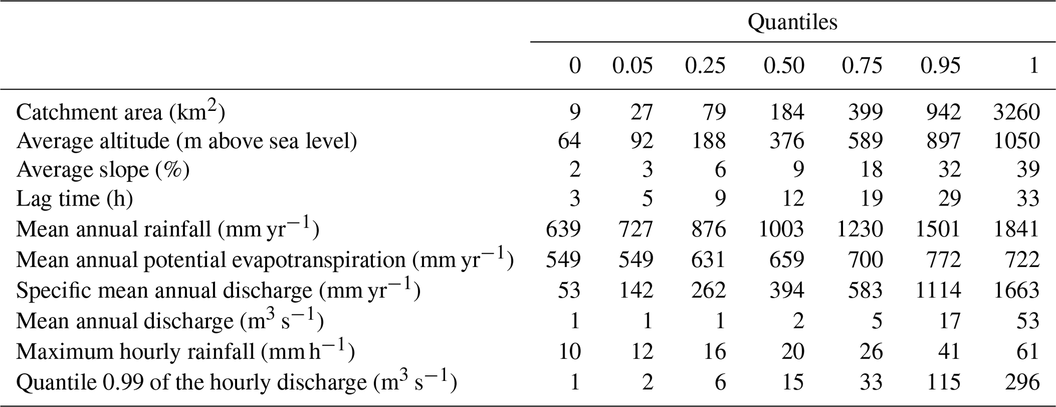
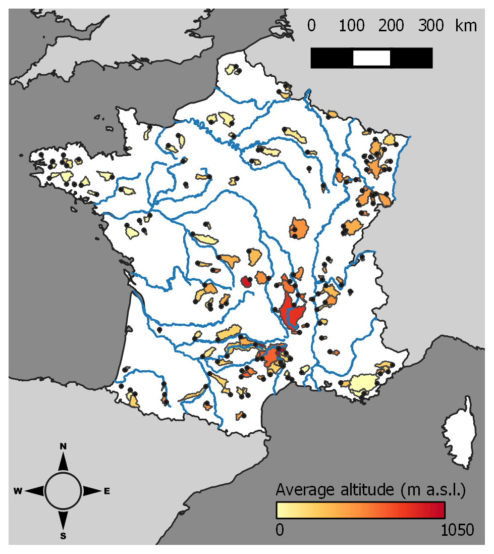
Download Print Version | Download XLSX

https://www.hydrol-earth-syst-sci.net/24/2017/2020/hess-24-2017-2020-f01

Figure 1The set of 154 unregulated catchments used in this study. Average altitude is given in metres above sea level (m a.s.l.).

2.1.2 Hydrological model

We used discharge forecasts computed by the GRP rainfall–runoff model. The GRP model is designed for flood forecasting and is currently used by the FFS in France in operational conditions (Furusho et al., 2016; Viatgé et al., 2018). It is a deterministic lumped storage-type model that uses catchment areal rainfall and PE as inputs. In forecasting mode (Appendix A), the model also assimilates discharge observations available when issuing a forecast to update the main state variable of the routing function and to update the output discharge. In this study, it is run at an hourly time step, and forecasts are issued for several lead times ranging from 1 to 72 h. More details about the GRP model can be found in Appendix A.

Since herein only the ability of the post-processor to extrapolate uncertainty quantification is studied, the model is fed only with observed rainfall (no forecast of precipitation), in order to reduce the impact of the input uncertainty. For the same reason, the model is calibrated in forecasting mode over the 10-year series by minimising the sum of squared errors for a lead time taken as the LT. The results will be presented for four lead times, – LT / 2, LT, 2 LT and 3 LT – to cover the different behaviours that can be seen when data assimilation is used to reduce errors in an operational flood forecasting context (Berthet et al., 2009).

2.1.3 Empirical hydrological uncertainty processor (EHUP)

We used the empirical hydrological uncertainty processor (EHUP) presented in Bourgin et al. (2014). It is a data-based and non-parametric approach in order to estimate the conditional predictive uncertainty distribution. This post-processor has been compared to other post-processors in earlier studies and proved to provide relevant results (Bourgin, 2014). It is now used by operational FFS in France under the operational tool called OTAMIN (Viatgé et al., 2019). The main difference with many other post-processors (such as the MCP, the meta-Gaussian processor, the BJP or the BFS) is that no assumption is made about the shape of the uncertainty distribution, which brings more flexibility to represent the various forecast error characteristics encountered in large-sample modelling. We will discuss the impact of this choice in Sect. 4.2.

The basic idea of the EHUP is to estimate empirical quantiles of errors stratified by different flow groups to account for the variation of the forecast error characteristics with forecast magnitude. Since forecast error characteristics also vary with the lead time when data assimilation is used, the EHUP is trained separately for each lead time.

For each lead time separately, the following steps are used:

Training:
- The flow groups are obtained by first ordering the forecast–observation pairs according to the forecasted values and then stratifying the pairs into a chosen number of groups (in this study, we used 20 groups), so that each group contains the same number of pairs.
- Within each flow group, errors are calculated as the difference between the two values of each forecast–observation pair, and several empirical quantiles (we used 99 percentiles) are calculated in order to characterise the distribution of the error values.
Application:
- The predictive uncertainty distribution that is associated with a given (deterministic) forecasted value is defined by adding this forecasted value to the empirical quantiles that belong to the same flow group as the forecasted value.

Since this study focuses on the extrapolation case, the validation is achieved with deterministic forecasts higher than the highest one used for the calibration. Therefore, only the highest-flow group of the calibration data is used to estimate the uncertainty assessment (to be used on the control data). This highest-flow group contains the top 5 % pairs of the whole training data, ranked by forecasted values. This threshold is chosen as a compromise between focusing on the highest values and using a sufficiently large number of forecast–observation pairs when estimating empirical quantiles of errors. In extrapolation, when the forecast discharge is higher than the highest value of the training period, the predictive distribution of the error is kept constant, i.e. the same values of the empirical quantiles of errors are used, as illustrated in Fig. 5.

The EHUP can be applied after a preliminary data transformation, and by adding a final step to back-transform the predictive distributions obtained in a transformed space. In previous work, we used the log transformation because it ensures that no negative values are obtained when estimating the predictive uncertainty for low flows (Bourgin et al., 2014). When estimating the predictive uncertainty for high flows, the data transformation has a strong impact in extrapolation, because the variation of the extrapolated predictive distribution, which is constant in the transformed space, is controlled in the real space by the behaviour of the inverse transformation, as explained below.

2.1.4 The different transformation families

Many uncertainty assessment methods mentioned in the Introduction use a variable transformation to handle the heteroscedasticity of the residuals and account for the variation of the prediction distributions with the magnitude of the predicted variable. Here, we briefly recall a number of variable transformations commonly used in hydrological modelling. Let y and $\tilde{y}$ be the observed and forecasted variables (here, the discharge), respectively, and $ε = y - \tilde{y}$ the residuals. When using a transformation g, we consider the residuals $ε^{'} = g (y) - g (\tilde{y})$ .

Three analytical transformations are often met in hydrological studies: the log, Box–Cox and log–sinh transformations. The log transformation is commonly used (e.g. Morawietz et al., 2011):

\begin{matrix} (1) & g_{1} : y \mapsto \log (y + a), \end{matrix}

where a is a small positive constant to deal with y values close to 0. It can be taken as equal to 0 when focusing on large discharge values. This transformation has no parameter to be calibrated. Applying a statistical model to residuals computed on log-transformed variables may be interpreted as using a corresponding model of multiplicative error (e.g. assuming a Gaussian model for residuals of log-transformed discharges is equivalent to a log-normal model of the multiplicative errors $y / \tilde{y}$ ). Therefore, it may be adapted to strongly heteroscedastic behaviours. It has been used successfully to assess hydrological uncertainty (Yang et al., 2007 b; Schoups and Vrugt, 2010; Bourgin et al., 2014).

The Box–Cox transformation (Box and Cox, 1964) is a classic transformation that is quite popular in the hydrological community (e.g. Yang et al., 2007 b; Wang et al., 2009; Hemri et al., 2015; Reichert and Mieleitner, 2009; Singh et al., 2013; Del Giudice et al., 2013):

\begin{matrix} (2) & g_{2 [λ]} : y \mapsto \frac{(y + a)^{λ} - 1}{λ} if λ \neq 0 and g_{2 [λ]} = g_{1} if λ = 0 . \end{matrix}

Here a is taken as being equal to 0 (as for the log transformation); the Box–Cox transformation is then a one-parameter transformation. It makes it possible to cover very different behaviours. The log transformation is a special case of the Box–Cox transformation when the calibration results in λ=0. In contrast, applying the Box–Cox transformation with λ=1 to the variable y to model the distribution of their residuals is equivalent to applying no transformation (Fig. 2). McInerney et al. (2017) obtained their most reliable and sharpest results with λ=0.2 over 17 perennial catchments.

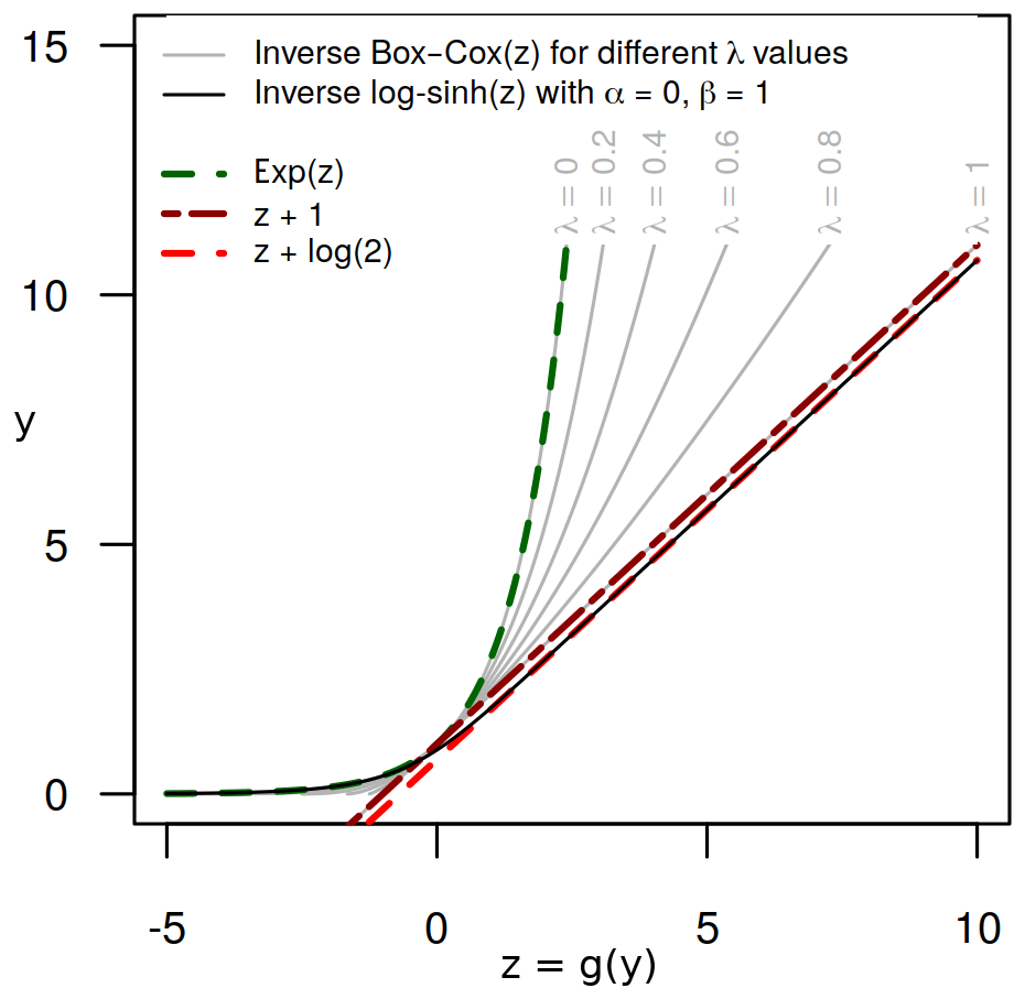
https://www.hydrol-earth-syst-sci.net/24/2017/2020/hess-24-2017-2020-f02

Figure 2The inverse transformation explains the final effect on the uncertainty assessment: the constant probability distribution in the transformed space (provided by the EHUP) will result in a distribution in the untransformed space, whose evolution depends on the behaviour of the inverse data transformation. Here, the Box–Cox transformation provides different behaviours, depending on its parameter value (λ). It ranges from an affine transformation (equivalent to no transformation; red dashed line) to the log transformation (thick green dashed line). With a single parameterisation, the log–sinh transformation can be equivalent to the log transformation for values of y much smaller than the value of its parameter β and equivalent to an affine transformation for large values of y (much higher than β; see Appendix B).

Download

More recently, the log–sinh transformation has been proposed (Wang et al., 2012; Pagano et al., 2013). It is a two-parameter transformation:

\begin{matrix} (3) & g_{3 [α, β]} : y \mapsto β \cdot \log (\sinh (\frac{α + y}{β})) . \end{matrix}

This transformation provides more flexibility. Indeed, for y≫α and y≫β, the log–sinh transformation reduces to no transformation, while for $α ≪ y ≪ β$ it is equivalent to the log transformation (Fig. 2). Thus, with the same parameterisation, it can result in very different behaviours depending on the magnitude of the discharge. Applying no transformation may be intuitively attractive when modelling the distribution of residuals for large discharge values when the variance is no longer expected to increase (homoscedastic behaviour). It is then particularly attractive when modelling predictive uncertainty in an extrapolation context, in order to avoid an excessively “explosive” assessment of the predictive uncertainty for large discharge values.

In addition to the log transformation used by Bourgin et al. (2014), in this study we tested the Box–Cox and the log–sinh transformations to explore more flexible ways to deal with the challenge of extrapolating prediction uncertainty distributions (Fig. 2). The impacts of the data transformations used in this study are illustrated in Fig. 3.

https://www.hydrol-earth-syst-sci.net/24/2017/2020/hess-24-2017-2020-f03

Figure 3Predictive 0.1 and 0.9 quantiles when assessed with no transformation, the log transformation, the Box–Cox transformation with its λ parameter equal to 0.5 and the log–sinh transformation with its α and β parameters equal to 0.1 and 8, on the Ill River at Didenheim (668 km²) for a lead time equal to LT, (a) as a function of the deterministic forecasted discharge and (b) for the flood event on 3 March 2006. The heteroscedasticity strongly differs from one variable transformation to another.

Download

Another common variable transformation is the normal quantile transformation (NQT; e.g. Kelly and Krzysztofowicz, 1997). It is a transformation without a calibrated parameter linking a given distribution and the Gaussian distribution, quantile by quantile. While several hydrological processors such as the HUP, MCP and QR encompass the NQT-transformed variables, Bogner et al. (2012) warn against the drawbacks of this transformation, which is by construction not suited for the extrapolation context and requires additional assumptions to model the tails of the distribution (Weerts et al., 2011; Coccia and Todini, 2011). This is why we did not test this transformation in this study focused on the extrapolation context.

2.2 Methodology: a testing framework designed for extrapolation context assessment

2.2.1 Testing framework

The EHUP is a non-parametric approach based on the characteristics of the distribution of residuals over a training data set. Moreover, the Box–Cox and the log–sinh transformations are parametric and require a calibration step. Therefore, the methodology adopted for this study is a split-sample scheme test inspired by the differential split-sample scheme of Klemes̆ (1986) and based on three data subsets: a data set for training the EHUP, a data set for calibrating the parameters of the variable transformation and a control data set for evaluating the predictive distributions when extrapolating high flows.

2.2.2 Events selection

To populate the three data subsets with independent data, separate flood events were first selected by an iterative procedure similar to those detailed by Lobligeois et al. (2014) and Ficchì et al. (2016): (1) the maximum forecasted discharge of the whole time series was selected; (2) within a 20 d period before (after) the peak flow, the beginning (end) of the event was placed at the preceding (following) time step closest to the peak at which the streamflow is lower than 20 % (25 %) of the peak flow value; and (3) the event was kept if there was less than 10 % missing values, if the beginning and end of the event were lower than 66 % of the peak flow value and if the peak value was higher than the median value of the time series. The process is then iterated over the remaining data to select all events. A minimum time lapse of 24 h was enforced between two events, ensuring that consecutive events are not overlapping and that the autocorrelation between the time steps of two separate events remains limited.

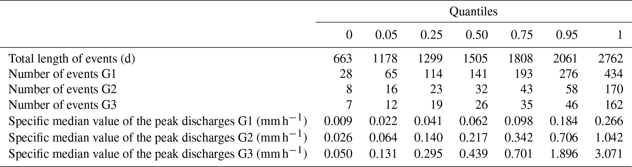
The number of events and their characteristics vary greatly among catchments, as summarised in Table 2. Note that the events selected for one catchment can slightly differ for the four different lead times considered in this study, because the selection was made using the forecasted discharge and not the observed discharge.

Table 2Characteristics of the events selected for the lead time (LT) over the 1997–2006 data series.

Download Print Version | Download XLSX

2.2.3 Selection of the data subsets

The selected events were then gathered into three events sets – G1, G2 and G3 – based on the magnitude of their peaks and the number of useful time steps for each test phase (training of the EHUP post-processor, calibration of the variable transformations and evaluation of the predictive distributions): G1 contains the lowest events, while the highest events are in G3.

The selection of the data subsets was tailored to study the behaviour of the post-processing approach in an extrapolation context. The control data subset had to encompass only time steps with simulated discharge values higher than those met during the training and calibration steps. Similarly, the calibration data subset had to encompass time steps with simulated discharge values higher than those of the training subset.

To achieve these goals, only the time steps within flood events were used. We distinguished four data subsets, as illustrated in Fig. 4. The subset D1 gathered all the time steps of the events of the G1 group. Then, the set D2 of the time steps of the events of the G2 group was split into two subsets: D2_sup gathered all the time steps with forecasted discharge values higher than the maximum met in D1, and D2_inf was filled with the other time steps. Finally, D3 was similarly filled with all the time steps of the G3 events with forecasted discharge values higher than the maximum met in D2.

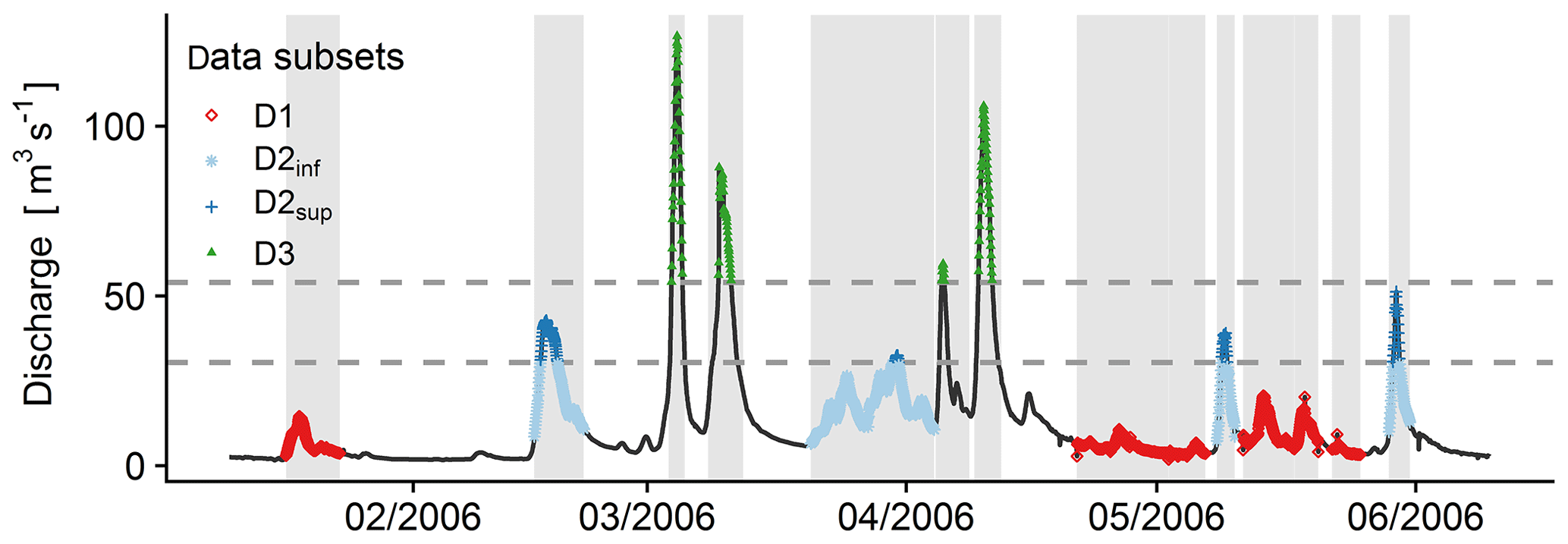
https://www.hydrol-earth-syst-sci.net/24/2017/2020/hess-24-2017-2020-f04

Figure 4Illustration of the selection of the data subsets for the Ill River at Didenheim (668 km²). First, the events are selected (grey highlighting). Then, the four data subsets are populated according to the thresholds (horizontal dashed lines). See Sect. 2.1.3 for more details.

Download

The discharge thresholds used to populate the D1, D2_sup and D3 subsets from the events belonging to the G1, G2 and G3 groups were chosen to ensure a sufficient number of time steps in every subset. We chose to set the minimum number of time steps in D3 and D2_sup to 720 as a compromise between having enough data to evaluate the methods and keeping the extrapolation range sufficiently large. We lowered this limit to 500 for the top 5 % pairs of D1, since this subset was only used to build the empirical distribution by estimating the percentiles during the training step and not used for evaluating the quality of the uncertainty assessment.

2.2.4 Calibration and evaluation steps

Since there are only one parameter for the Box–Cox transformation and two parameters for the log–sinh transformation, a simple calibration approach of the transformation parameters was chosen: the parameter space was explored by testing several parameter set values. For the Box–Cox transformation, 17 values for the λ parameter were tested: from 0 to 1 with a step of 0.1 and with a refined mesh for the sub-intervals 0–0.1 and 0.9–1. For the log–sinh transformation, a grid of 200 (α, β) values was designed for each catchment based on the maximum value of the forecasted discharge in the D2 subset, as explained in greater detail in Appendix B.

Note that the hydrological model was calibrated over the whole set of data (1997–2006) to make the best use of the data set, since this study focuses on the effect of extrapolation on the predictive uncertainty assessment only.

We used a two-step procedure, as illustrated in Fig. 5. The first step was to calibrate the parametric transformations. For each transformation and for each parameter set, the empirical residuals were computed over D1 and D2_sup, where the EHUP was trained on the highest-flow group of D1 (see Sect. 2.1.3) and the calibration criterion was computed on D2_sup. Indeed, the data transformations have almost no impact on the uncertainty estimation by EHUP for events of the same magnitude as those of the training subset. Therefore, the calibration subset has to encompass events of a larger magnitude (D2_sup). The parameter set obtaining the best criterion value was selected. In the second step, the EHUP was trained on the highest-flow group of D1, D2_inf and D2_sup combined and using the parameter set obtained during the calibration step. Then, the predictive uncertainty distribution was evaluated on the control data set D3. Training the EHUP on the highest-flow group of the union of D1, D2_inf and D2_sup allows the uncertainty assessment to be controlled from small to large degrees of extrapolation (on D3). Indeed if we had kept the training on D1 only, we would have not been able to test small degrees of extrapolation on independent data for every catchment (see the discussion in Sect. 3.3).

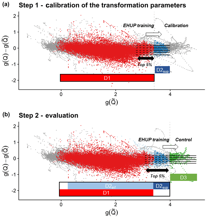
https://www.hydrol-earth-syst-sci.net/24/2017/2020/hess-24-2017-2020-f05

Figure 5Residuals as a function of the forecast discharges in the transformed space. The horizontal dashed lines represent the 0.1, 0.25, 0.5, 0.75 and 0.9 quantiles of the residuals computed during the training phase of the EHUP post-processor, for the highest-flow group (top 5 % pairs of the training data ranked by forecasted values). The straight horizontal lines represent their use in assessing the predictive uncertainty in extrapolation during (a) the calibration step of the variable transformation parameters and (b) the evaluation step of the predictive uncertainty. During the calibration step (a), many parameters set values are tested, while only the calibrated set of transformation parameters is used during the evaluation step (b). The vertical dashed lines show the beginning of the extrapolation range. The grey dots are the data pairs which are not selected in D1, D2_inf, D2_sup or D3: they are not used during the calibration step or the evaluation step. Illustration from the Ill River at Didenheim, 668 km². Data used for the EHUP training at each step is sketched by a thick rectangle. In this study, only the top 5 % pairs of the training data ranked by forecasted values are used to estimate the residual distribution, since we focus on the extrapolation behaviour of the EHUP.

Download

2.3 Performance criteria and calibration

2.3.1 Probabilistic evaluation framework

Reliability was first assessed by a visual inspection of the probability integral transform (PIT) diagrams (Laio and Tamea, 2007; Renard et al., 2010). Since this study was carried out over a large sample of catchments, two standard numerical criteria were used to summarise the results: the α index, which is directly related to the PIT diagram (Renard et al., 2010), and the coverage rate of the 80 % predictive intervals (bounded by the 0.1 and 0.9 quantiles of the predictive distributions), used by the French operational FFS (a perfect uncertainty assessment would reach a value of 0.8). The α index is equal to $1 - 2 \cdot A$ , where A is the area between the PIT curve and the bisector, and its value ranges from 0 to 1 (perfect reliability).

The overall quality of the probabilistic forecasts was evaluated with the continuous rank probability score (CRPS; Hersbach, 2000), which compares the predictive distribution to the observation:

\begin{matrix} (4) & CRPS = \frac{1}{N} \sum_{k = 1}^{N} \int_{0}^{+ \infty} {[F_{k} (Q) - H (Q - Q_{k, obs})]}^{2} d Q, \end{matrix}

where N is the number of time steps, F(Q) is the predictive cumulative distribution, H the Heaviside function and Q_obs is the observed value. We used a skill score (CRPSS) to compare the mean CRPS to a reference, here the mean CRPS obtained from the unconditional climatology, i.e. from the distribution of the observed discharges over the same data subset. Values range from −∞ to 1 (perfect forecasts): a positive value indicates that the modelling is better than the climatology.

For operational purposes, the sharpness of the probabilistic forecasts was checked by measuring the mean width of the 80 % predictive intervals. A dimensionless relative-sharpness index was obtained by dividing the mean width by the mean runoff:

\begin{matrix} (5) & 1 - \frac{\sum_{k = 1}^{N} [q_{0.9} (Q_{k}) - q_{0.1} (Q_{k})]}{\sum_{k = 1}^{N} Q_{k, obs}}, \end{matrix}

where q₉₀(Q) and q₁₀(Q) are the upper and the lower bounds of the 80 % predictive interval for each forecast, respectively. The sharper the forecasts, the closer this index is to 1.

In addition to the probabilistic criteria presented above, the accuracy of the forecasts was assessed using the Nash–Sutcliffe efficiency (NSE) calculated with the mean values of the predictive distributions (best value: 1).

2.3.2 The calibration criterion

Since the calibration step aims at selecting the most reliable description of the residuals in extrapolation, the α index was used to select the parameter set that yields the highest reliability for each catchment, each lead time and each transformation. While other choices were possible, we followed the paradigm presented by Gneiting et al. (2007): reliability has to be ensured before sharpness. Note that the CRPS could have been chosen, since it can be decomposed as the sum of two terms: reliability and sharpness (Hersbach, 2000). However, in the authors' experience, the latter is the controlling factor (Bourgin et al., 2014). Moreover, the CRPS values were often quite insensitive to the values of the log–sinh transformation parameters.

In cases where an equal value of the α index was obtained, we selected the parameter set that gave the best sharpness index. For the log–sinh transformation, there were still a few cases where an equal value of the sharpness index was obtained, revealing the lack of sensitivity of the transformation in some areas of the parameter space. For those cases, we chose to keep the parameter set that had the lowest α value and the β value closest to $\max_{D 2} (\tilde{Q})$ .

https://www.hydrol-earth-syst-sci.net/24/2017/2020/hess-24-2017-2020-f06

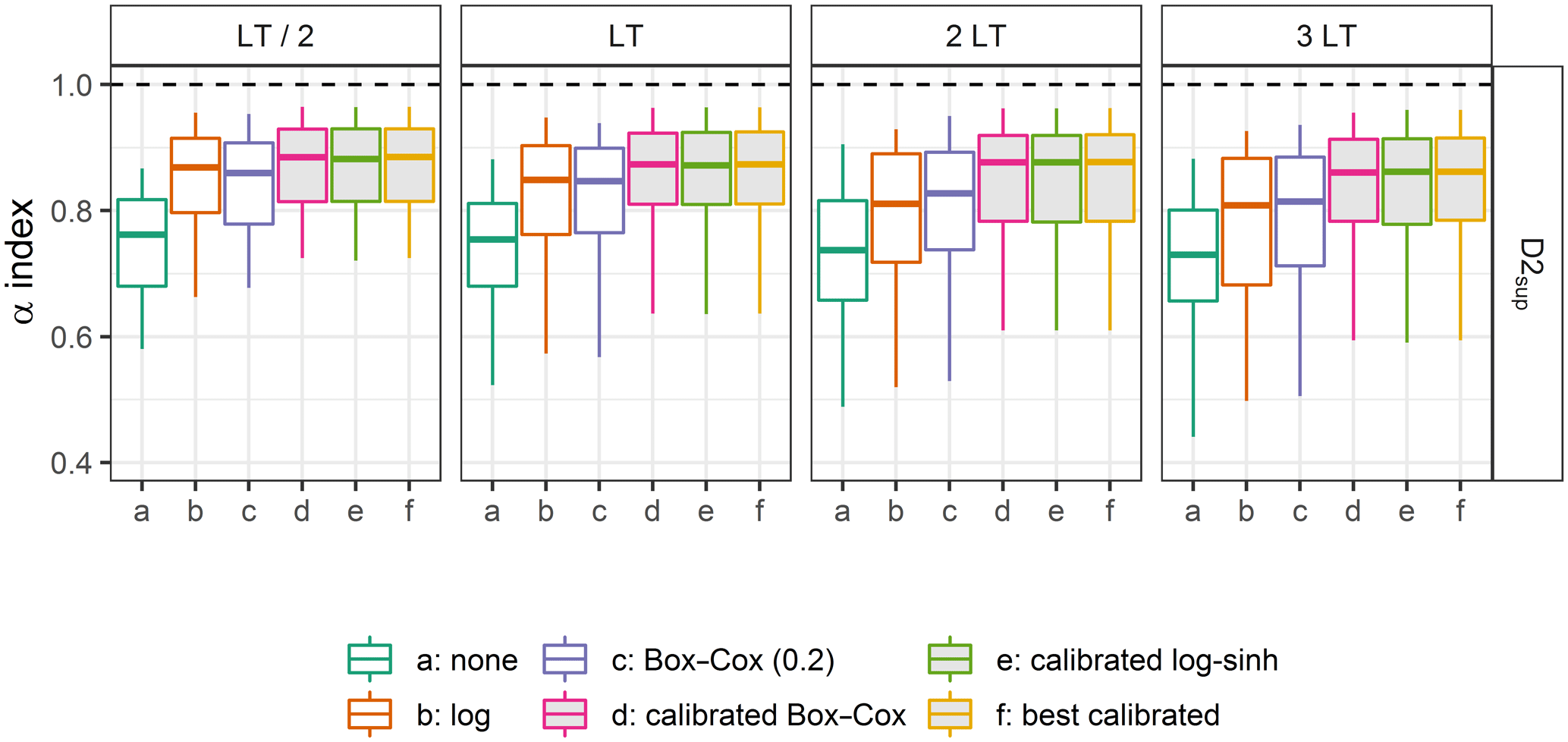
Figure 6Distributions of the α-index values on the calibration data set D2_sup, obtained with different transformations for four lead times (the filled box plots represent the calibrated distributions). Box plots (5th, 25th, 50th, 75th and 95th percentiles) synthesise the variety of scores over the catchments of the data set. The optimal value is represented by the horizontal dashed lines.

Download

https://www.hydrol-earth-syst-sci.net/24/2017/2020/hess-24-2017-2020-f07

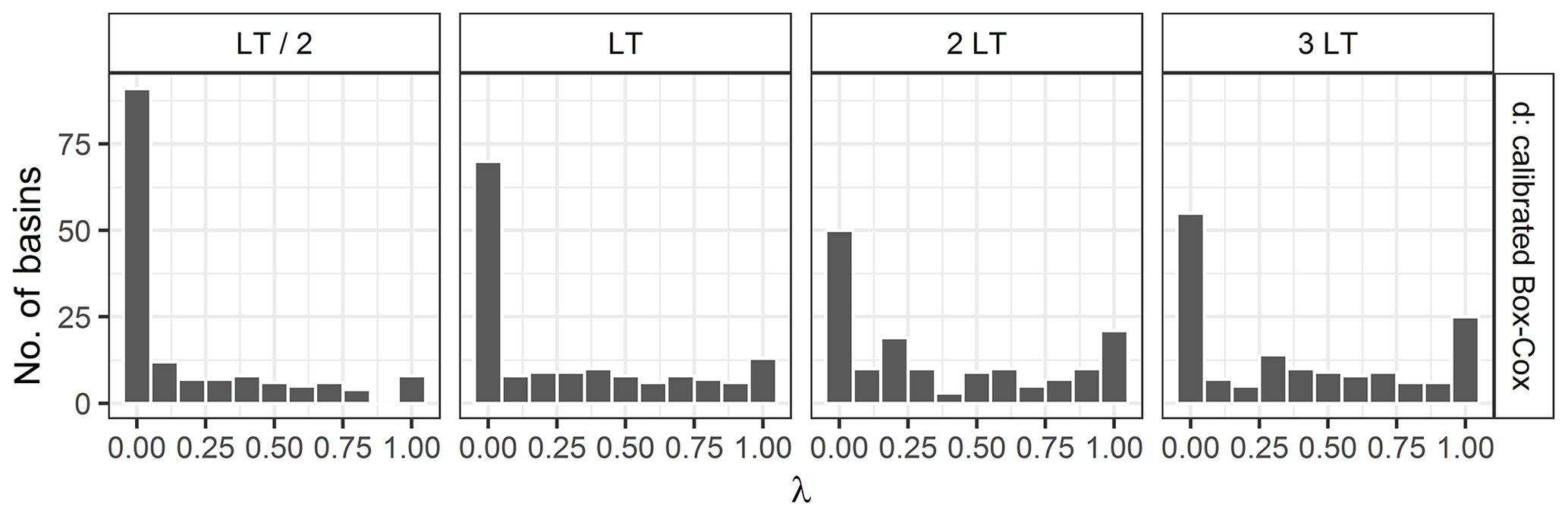
Figure 7Distribution over the basins of the values of the Box–Cox transformation parameter obtained during the calibration step for the four different lead times.

Download

3 Results

3.1 Results with the calibration data set D2_sup

Figure 6 shows the distributions of the α-index values obtained with different transformations on the calibration data set (D2_sup) for lead times LT / 2, LT, 2 LT and 3 LT. The distributions are summarised with box plots. Clearly, not using any transformation leads to poorer reliability than any tested transformation. In addition, we note that the calibrated transformations provide better results (although not perfect) than the uncalibrated ones in the calibration data set, as expected, and that no noticeable difference can be seen in Fig. 6 between the calibrated Box–Cox transformation (d), the calibrated log–sinh transformation (e) and the best-calibrated transformation (f). Nevertheless, the uncalibrated log transformation and Box–Cox transformation with parameter λ set at 0.2 (BC_λ=0.2) reach quite reliable forecasts. Comparing the results obtained for the different lead times reveals that less reliable predictive distributions are obtained for longer lead times, in particular for the transformations without a calibrated parameter.

Figures 7 and 8 show the distribution of parameter values obtained for the Box–Cox and the log–sinh transformation during the calibration step. The distributions vary with lead time. While the log transformation behaviour is frequently chosen for LT/2 and LT, the additive behaviour (corresponding to the use of no transformation; see Sect. 2.1.4) becomes more frequent for 2 and 3 LT. A similar conclusion can be drawn for the log–sinh transformation: a low value of α and a high value of β yield a multiplicative behaviour that is frequently chosen, for all lead times, but less for 2 and 3 LT than for LT/2 and LT. This explains in particular the loss of reliability that can be seen for the log transformation for 3 LT in Fig. 6. These results reveal that the extrapolation behaviour of the distributions of residuals is complex. It varies among catchments and with lead time because of the strong impact of data assimilation.

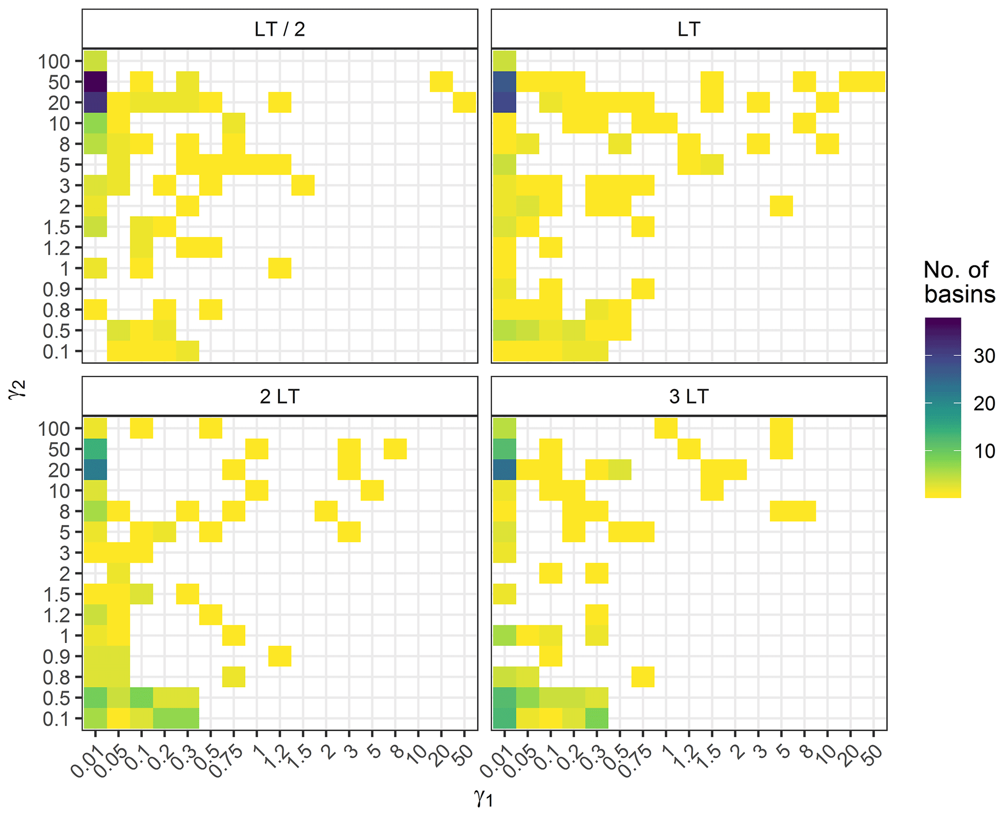
https://www.hydrol-earth-syst-sci.net/24/2017/2020/hess-24-2017-2020-f08

Figure 8Distribution over the basins of the values of the log–sinh transformation parameters obtained during the calibration step for the four different lead times. $γ_{1} = α / \max_{D 2} (\tilde{Q})$ and $γ_{2} = β / \max_{D 2} (\tilde{Q})$ (see Appendix B).

Download

3.2 Results with the D3 control data set

3.2.1 Reliability

First, we conducted a visual inspection of the PIT diagrams, which convey an evaluation of the overall reliability of the probabilistic forecasts (examples in Fig. 9). In some cases, the forecasts are reliable (e.g. the Thérain River at Beauvais, 755 km², except if no transformation is used). Alternatively, these diagrams may show quite different patterns, highlighting bias (e.g. the Meu River at Montfort-sur-Meu, 477 km²) or under-dispersion (e.g. the Aa River at Wizernes, 392 km², or the Sioulet River at Miremont, 473 km²; for the latter, the calibration on D2_sup leads to log–sinh and Box–Cox transformations equivalent to no transformation, which turns out not to be relevant for the control data set, where the log and the Box–Cox transformations are more reliable).

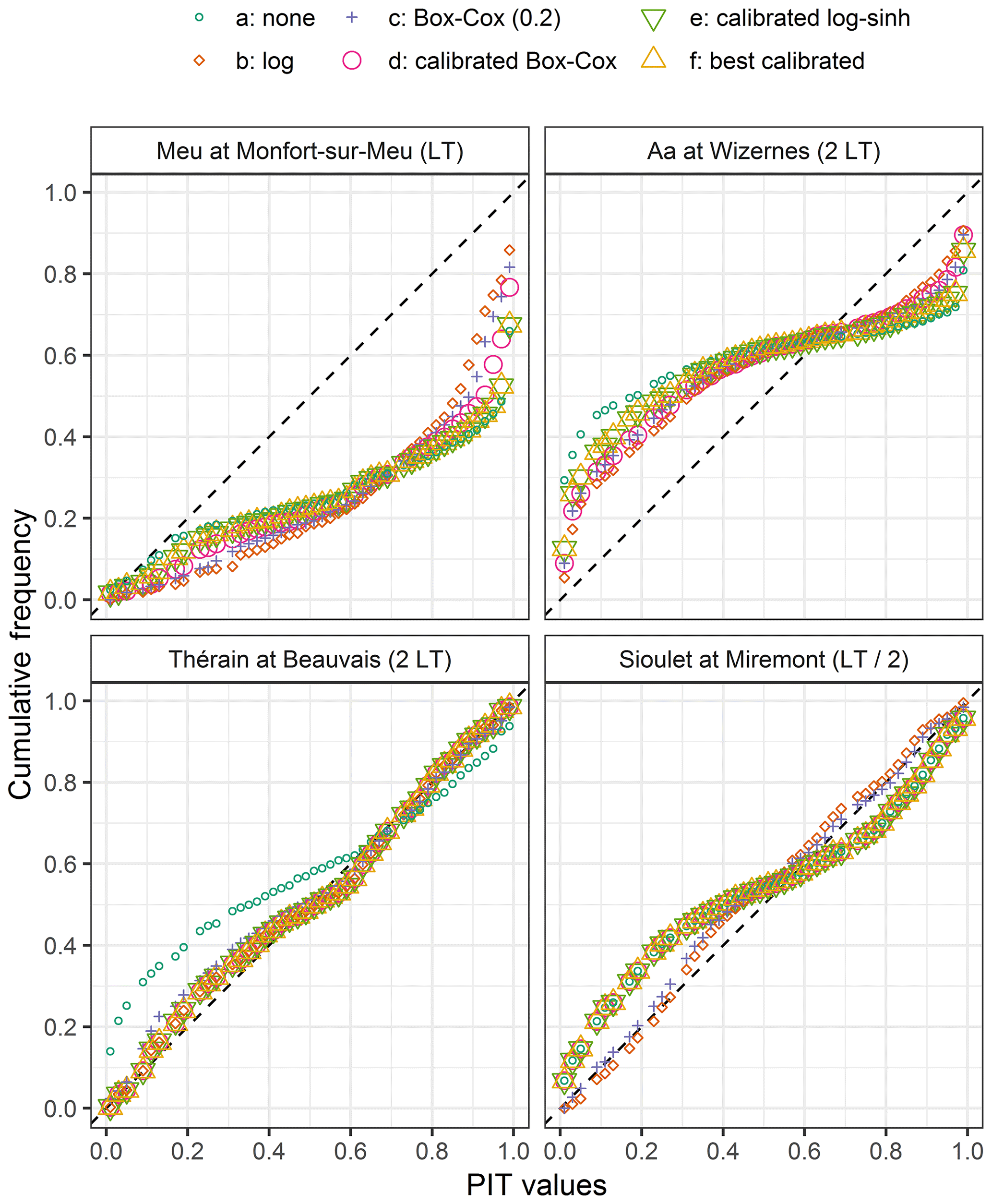
https://www.hydrol-earth-syst-sci.net/24/2017/2020/hess-24-2017-2020-f09

Figure 9Examples of PIT diagrams obtained with the control data set D3, with different transformations at four locations.

Download

Then the distribution of the α-index values in Fig. 10 reveals a significant loss of reliability compared to the values obtained with the calibration data set (Fig. 6). We note that the log transformation is the most reliable approach for LT / 2 and is comparable to the Box–Cox transformation (BC_λ=0.2) for LT. With increasing lead time, the BC_λ=0.2 transformation becomes slightly better than the other transformations, including the calibrated ones. In addition, comparing the results obtained for the different lead times confirms that it is challenging to produce reliable predictive distributions when extrapolating at longer lead times. Overall, it means that the added value of the flexibility brought by the calibrated transformations is not transferable in an independent extrapolation situation, as illustrated in Fig. 11.

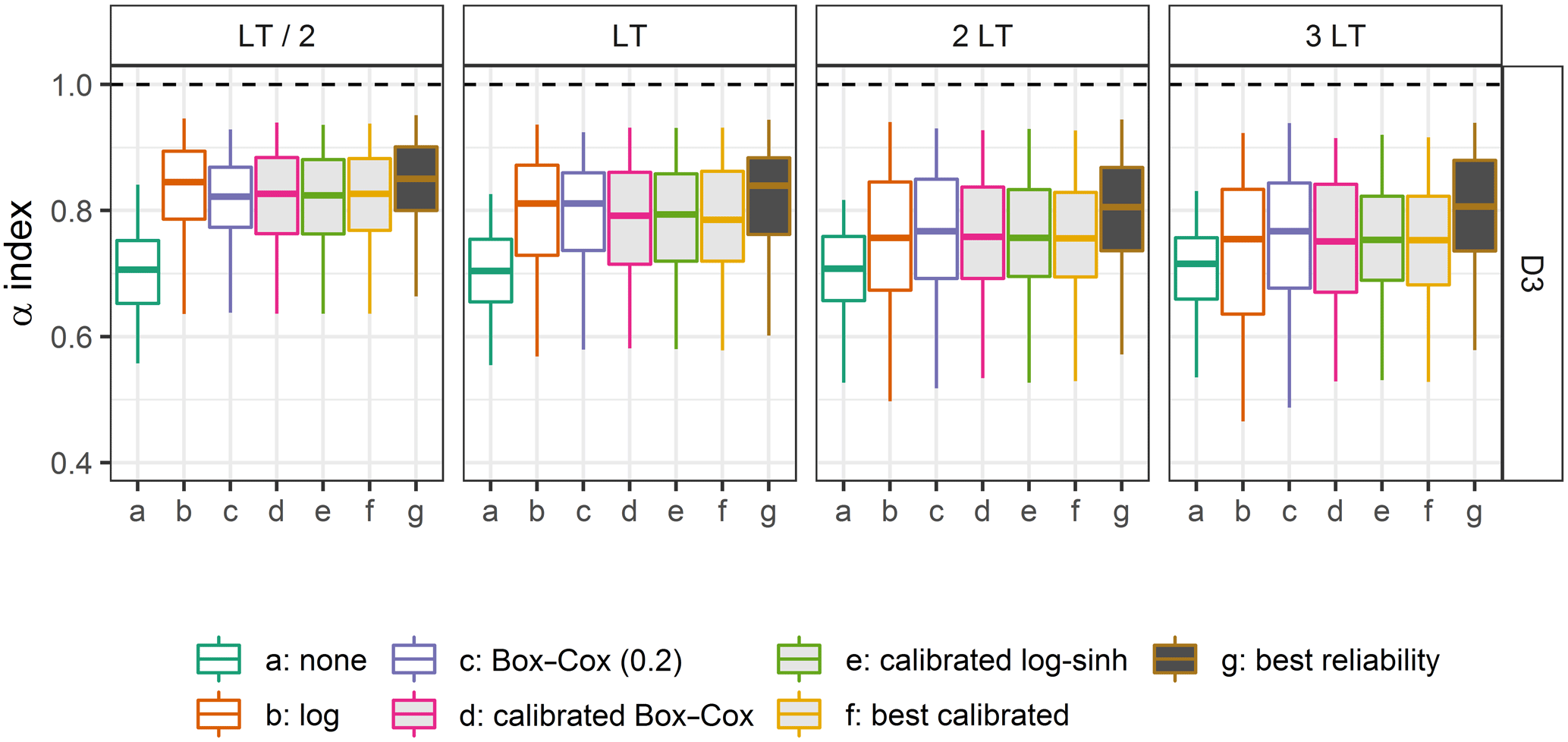
https://www.hydrol-earth-syst-sci.net/24/2017/2020/hess-24-2017-2020-f10

Figure 10Distributions of the α-index values on the control data set D3, obtained with different transformations for four lead times (the filled box plots represent the calibrated distributions). Box plots (5th, 25th, 50th, 75th and 95th percentiles) synthesise the variety of scores over the catchments of the data set. The optimal values are represented by the horizontal dashed lines. Option “g” gives the best performance that could be achieved with this model and this post-processor for these catchments (see the discussion in Sect. 4.1).

Download

https://www.hydrol-earth-syst-sci.net/24/2017/2020/hess-24-2017-2020-f11

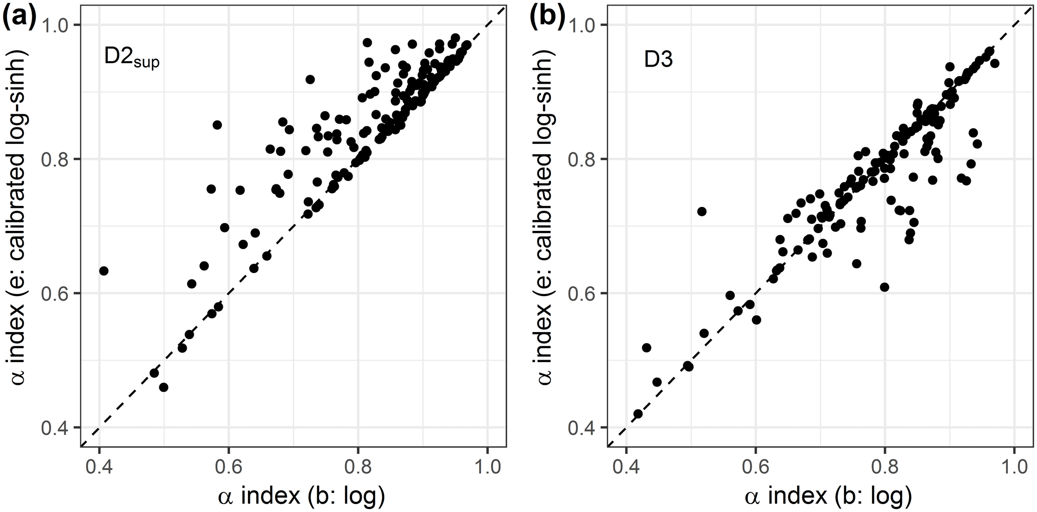
Figure 11Scatter plots of the reliability α index obtained with the log transformation and the log–sinh transformation (a) in D2_sup on the calibration step and (b) on D3 in the control step.

Download

In operational settings, non-exceedance frequencies of the quantiles of the predictive distribution, which are the lower and upper bounds of the predictive interval communicated to the authorities, are of particular interest. The 80 % predictive interval (bounded by the 0.1 and 0.9 quantiles) is mostly used in France. It is expected that the non-exceedance frequency of the lower bound and the exceedance frequency of the upper bound remain close to 10 % for a reliable predictive distribution. Deviations from these frequencies indicate biases in the estimated quantiles. Figure 12 reveals that on average the 0.1 quantile is generally better assessed than the 0.9 quantile on average, though the latter is generally more sought after for operational purposes. More importantly, the lack of reliability of the log transformation for the 3 LT lead time seen in Fig. 10 appears to be related to an underestimation of the 0.1 quantile, which is higher than for the other tested transformations, while the 0.9 quantile is less underestimated than for the other transformations. These results highlight that reliability can have different complementary facets and that some parts of the predictive distributions can be more or less reliable. In a context of flood forecasting, particular attention should be given to the upper part of the predictive distribution.

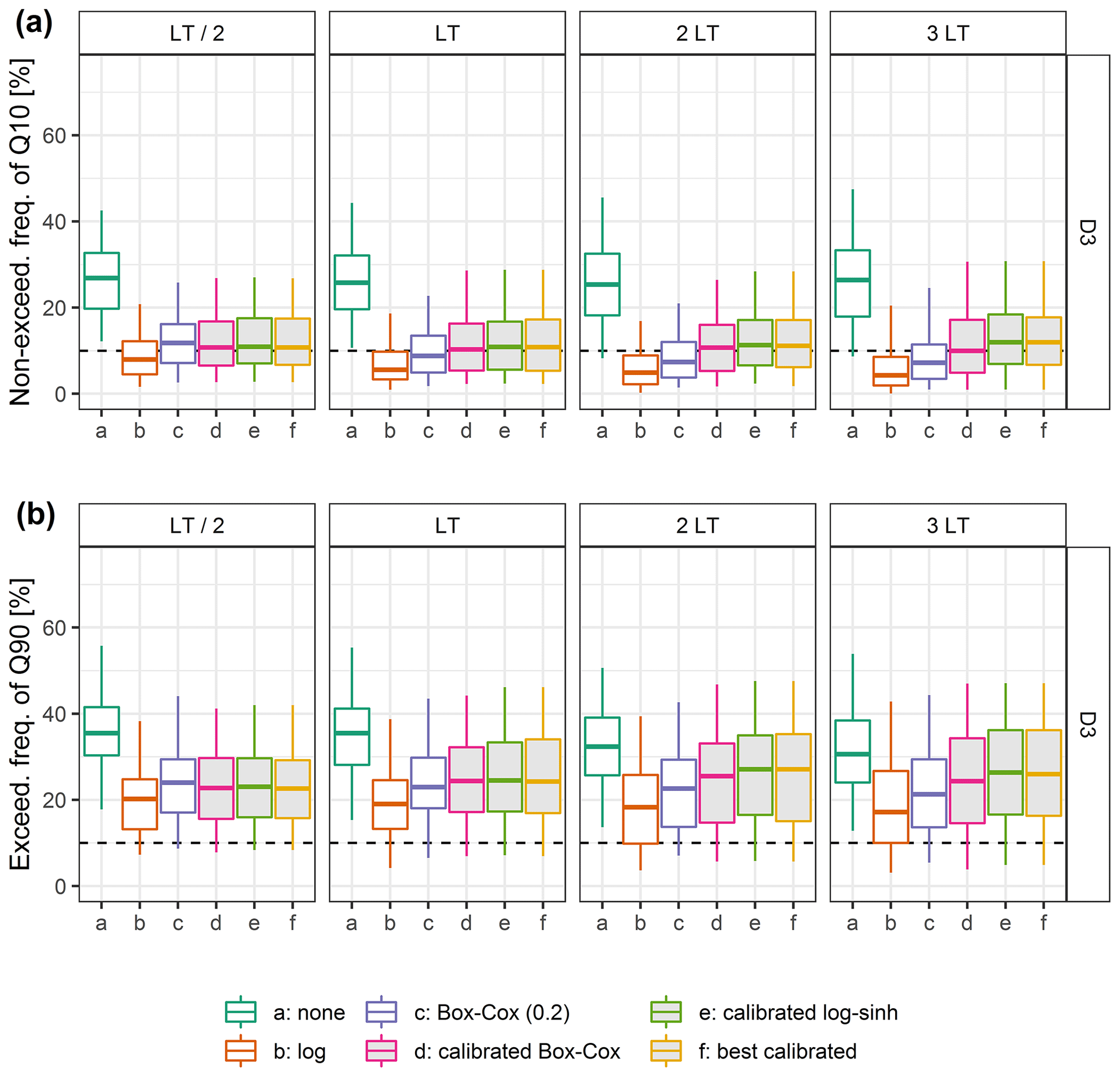
https://www.hydrol-earth-syst-sci.net/24/2017/2020/hess-24-2017-2020-f12

Figure 12Distributions over the catchment set of (a) the non-exceedance frequency of the 0.1 quantile and (b) the exceedance frequency of the 0.9 quantile on the control data set D3, obtained with the different transformations tested (the filled box plots are related to calibrated transformations). The optimal values are represented by the horizontal dashed lines.

Download

3.2.2 Other performance metrics

In addition to reliability, we looked at other qualities of the probabilistic forecasts, namely the overall performance (measured by the CRPSS) and accuracy (measured by NSE). We also checked their sharpness (relative-sharpness metric). The distributions of four performance criteria are shown for LT in Fig. 13. We note that the log transformation has the closest median value for the coverage ratio, at the expense of a lower median relative-sharpness value, because of larger predictive interval widths caused by the multiplicative behaviour of the log transformation. In addition, the CRPSS and the NSE distributions have limited sensitivity to the variable transformation (also shown by Woldemeskel et al. (2018) for the CRPS), even if we can see that not using any transformation yields slightly better results. This confirms that the CRPSS itself is not sufficient to evaluate the adequacy of uncertainty estimation. Similar results were obtained for the other lead times (Supplement).

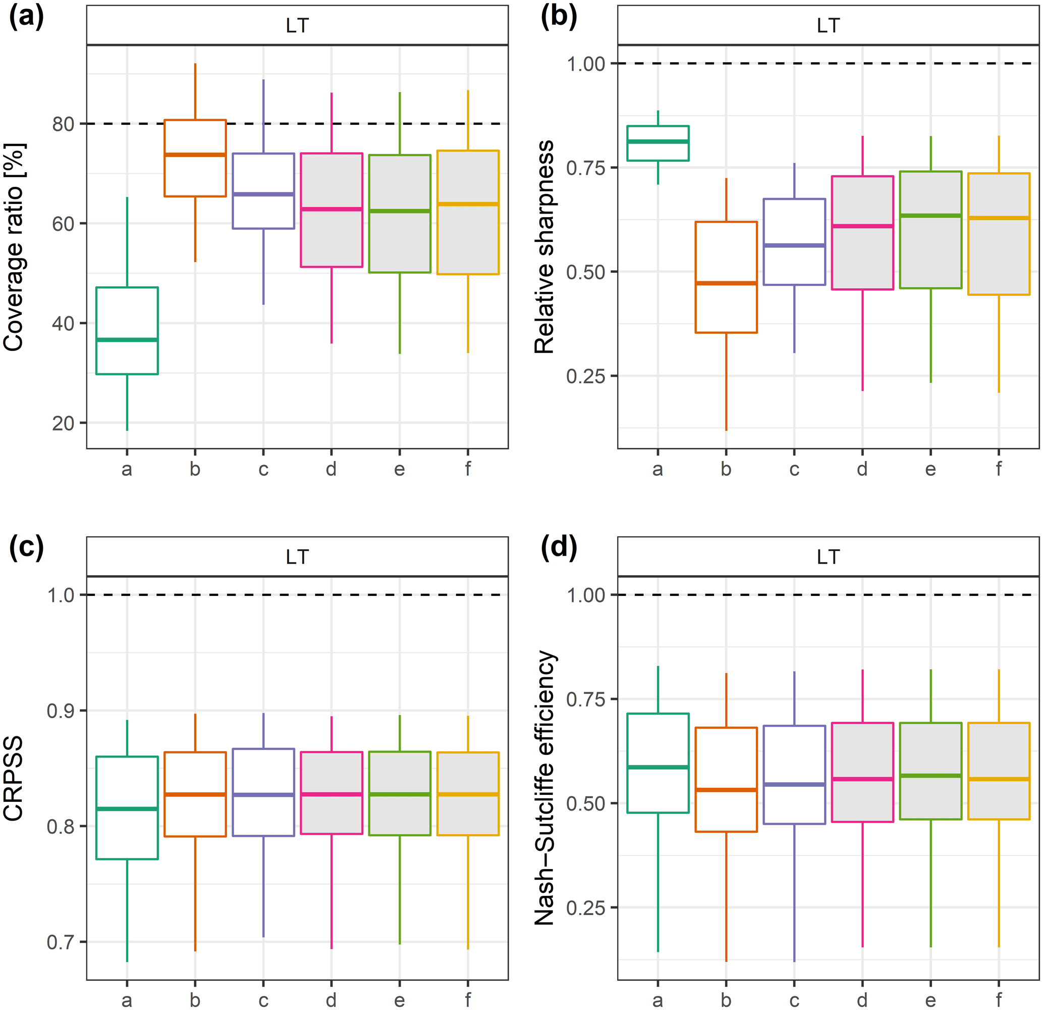
https://www.hydrol-earth-syst-sci.net/24/2017/2020/hess-24-2017-2020-f13

Figure 13Distributions of coverage rate, relative-sharpness, CRPSS and NSE values over the catchment set on the control data set D3, obtained with the different transformations tested (the filled box plots are related to calibrated transformations). The optimal values are represented by the horizontal dashed lines.

Download

3.3 Investigating the performance loss in an extrapolation context

For operational forecasters, it is important to be able to predict when they can trust the forecasts issued by their models and when their quality becomes questionable. Therefore we investigated whether the reliability and reliability loss observed in an extrapolation context were correlated with some properties of the forecasts. First, Fig. 14 shows the relationship between the α-index values obtained with D2_sup and those obtained with D3 for three representative transformations. The results indicate that it is not possible to anticipate the α-index values when extrapolating high flows in D3 based on the α-index values obtained when extrapolating high flows in D2_sup.

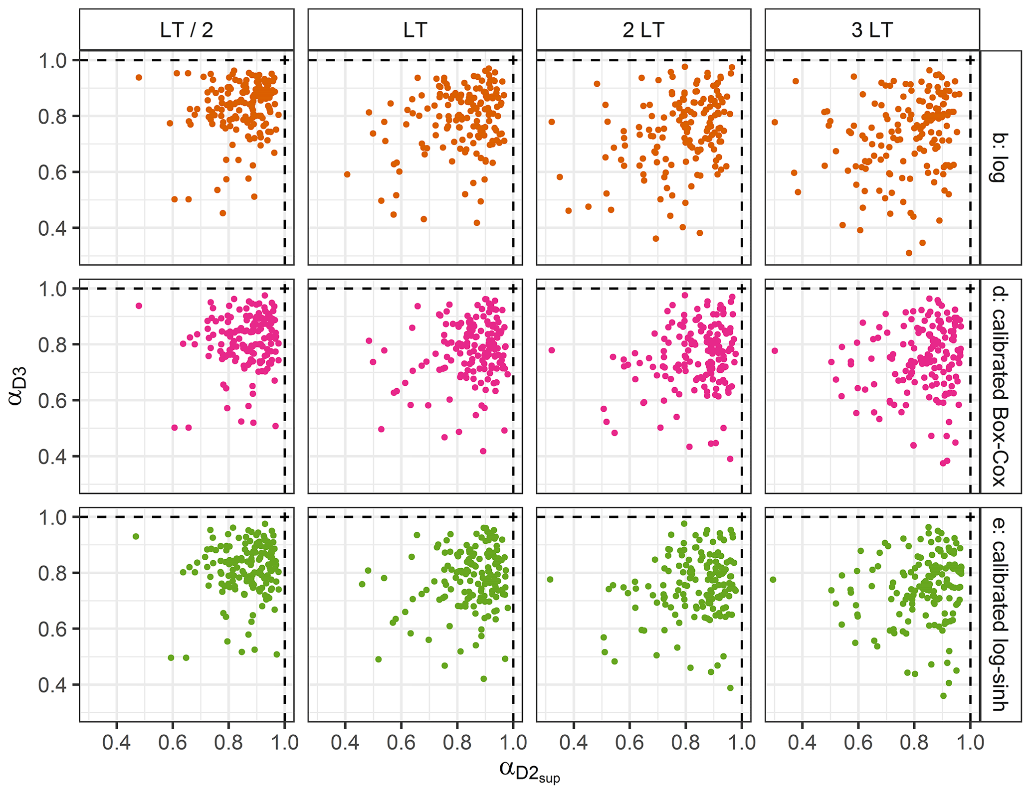
https://www.hydrol-earth-syst-sci.net/24/2017/2020/hess-24-2017-2020-f14

Figure 14Comparison of the α-index values obtained with D2_sup and D3. One point for each catchment. The optimal values are represented by the dashed lines. Similar results were obtained for the three other transformations (not shown).

Download

In addition, two indices were chosen to describe the degree of extrapolation: the ratio of the median of the forecasted discharges in D3 over the median of the forecasted discharge in D2_sup, and the ratio of the median of the forecasted discharges in D3 over the discharge for a return period of 20 years (for catchments where the assessment of the vicennial discharge was available in the national database: http://www.hydro.eaufrance.fr, last access: March 2020). In both cases, no trend appears, regardless of the variable transformation used, with Spearman coefficients values (much) lower than 0.33. The reliability can remain high for some catchments even when the magnitude of the events of the control data set is much higher than that of the training data set (see Supplement for figures).

Finally, we found no correlation with the relative accuracy of the deterministic forecasts either. The goodness of fit during the calibration phase cannot be used as an indicator of the robustness of the uncertainty estimation in an extrapolation context (see Supplement for figures).

4 Discussion

4.1 Do more complex parametric transformations yield better results in an extrapolation context?

Overall, the results obtained for the control data set suggest that the log transformation and the fixed Box–Cox transformation (BC_λ=0.2) can yield relatively satisfactory α index and coverage ratio values given their multiplicative or near-multiplicative behaviour in extrapolation. More tapered behaviours that can be obtained with the calibrated Box–Cox or log–sinh transformations do not show advantages when extrapolating high flows on an independent data set. In other words, what is learnt during the calibration of the more complex parametric transformations does not yield better results in an extrapolation context.

These results could be explained by the fact that the calibration did not result in the optimally relevant parameter set. To investigate whether another calibration strategy could yield better results, we compared the performance on the control D3 data set when the calibration is achieved on the D2_sup data set (“f: best calibrated”) and on the D3 data set (“g: best reliability”). The results shown in Fig. 10 reveal that, even when the best parameter set is chosen among the 217 possibilities tested in this study (17 for the Box–Cox transformation and 200 for the log–sinh transformation), the α-index distributions are far from perfect and reliability decreases with increasing lead time. This suggests that the stability of the distributions of residuals when extrapolating high flows might be a greater issue than the choice of the variable transformation. Nonetheless, the gap between the distributions of the transformations without a calibrated parameter (“b” and “c”), the best-calibrated transformation (“f”) and the best performance that could be achieved (“g”) highlights that it might be possible to obtain better results with a more advanced calibration strategy. This is, however, beyond the scope of this study and is therefore left for further investigations.

4.2 Empirically based versus distribution-based approaches: does the distribution shape choice impact the uncertainty assessment in an extrapolation context?

Besides the reduction of heteroscedasticity, many studies use post-processors which are explicitly based on the assumption of a Gaussian distribution and use data transformations to fulfil this hypothesis (Li et al., 2017). Examples are the MCP or the meta-Gaussian model; the NQT was designed to precisely achieve it. In their study on autoregressive error models used as post-processors, Morawietz et al. (2011) showed that error models with an empirical distribution for the description of the standardised residuals perform better than those with a normal distribution. We first checked whether the variable transformation helped to reach a Gaussian distribution of the residuals computed with the transformed variables. Then we investigated whether better performance can be achieved using empirical transformed distributions of residuals or using Gaussian distributions calibrated on these empirical distributions.

We used the Shapiro–Francia test where the null hypothesis is that the data are normally distributed. For each parametric transformation, we selected the parameter set of the calibration grid which obtains the highest p value. For more than 98 % of the catchments, the p value is lower than 0.018 (0.023) when the Box–Cox transformation (the log–sinh transformation) is used. This indicates that there are only a few catchments for which the normality assumption is not to be rejected. In a nutshell, the variable transformations can stabilise the variance, but they do not necessarily ensure the normality of the residuals. It is important not to overlook this frequently encountered issue in hydrological studies.

Even if there is no theoretical advantage to using the Gaussian distribution calibrated on the transformed-variable residuals rather than the empirical distribution to assess the predictive uncertainty, we tested the impact of this choice. For each transformation, the predictive uncertainty assessment obtained with the empirical transformed-variable distribution of residuals is compared to the assessment based on the Gaussian distribution whose mean and variance are those of the empirical distribution. Figure 15 shows the α-index distributions obtained over the catchments for both options in the control data set D3. We note that no clear conclusion can be drawn. No transformation (or identity transformation), which does not reduce the heteroscedasticity at all, benefits from the use of the Gaussian distributions for all lead times. In contrast, the predictive uncertainty assessment based on the empirical distribution with the log transformation is more reliable than the one based on the Gaussian distribution. For short lead times, it is slightly better to use the empirical distributions for the calibrated transformations (Box–Cox and log–sinh), but we observe a different behaviour for longer lead times. For these longer lead times, assessing the predictive uncertainty using the Gaussian distribution fitted to the empirical distributions of transformed residuals obtained with the calibrated log–sinh or Box–Cox transformations is the most reliable option. It is better than using the log transformation with the empirical distribution, but not very different from using the BC_λ=0.2 transformation.

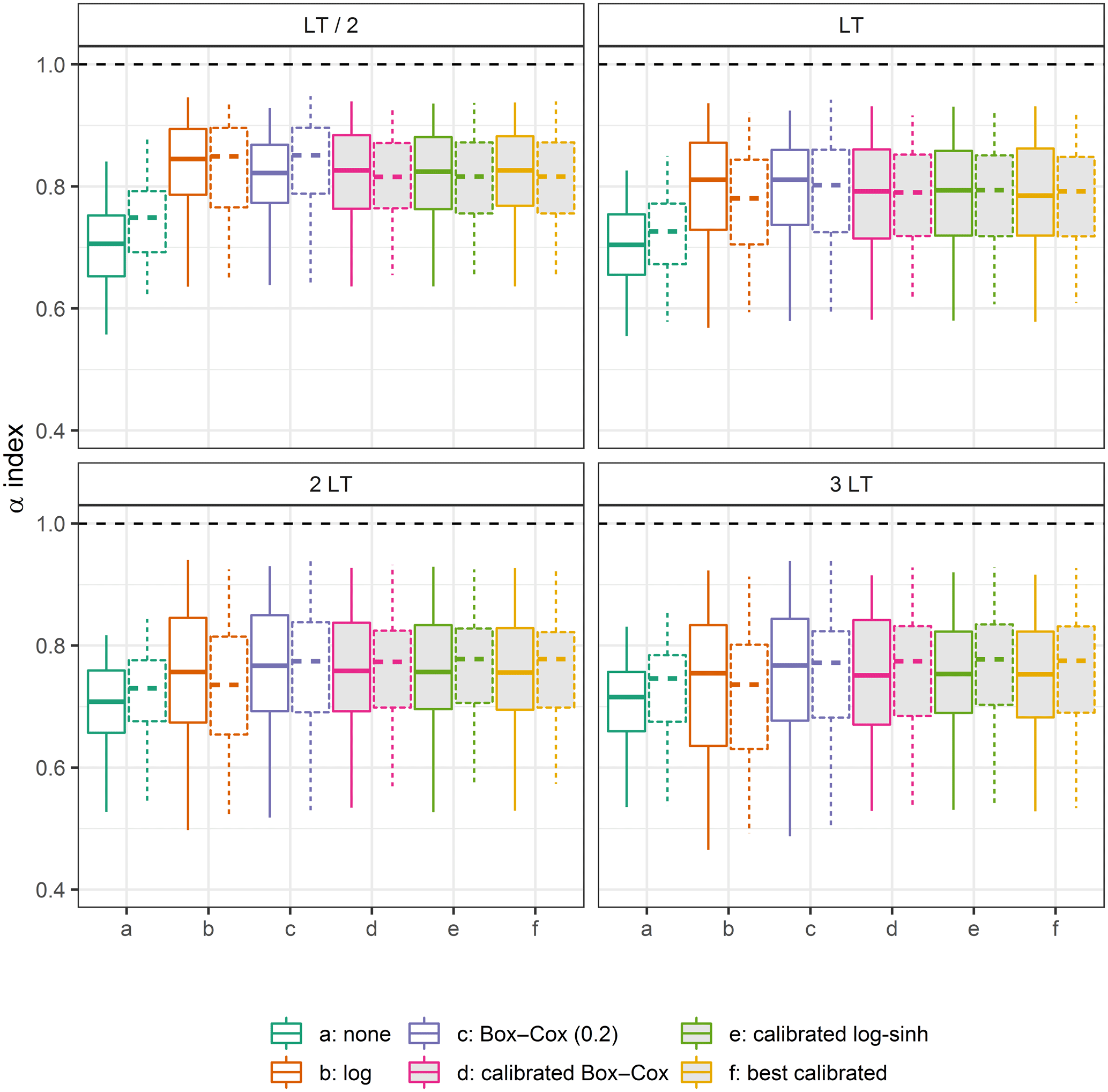
https://www.hydrol-earth-syst-sci.net/24/2017/2020/hess-24-2017-2020-f15

Figure 15Distributions of the α-index values on the control data set D3, obtained with different transformations for four lead times, when using the empirical distributions of residuals (straight box plots) and the Gaussian distributions (dashed box plots). The optimal values are represented by the horizontal dashed lines.

Download

Investigations on the impact of the choice between the empirical and the Gaussian distributions on the post-processor performance are shown in the Supplement. They show that the choice of the distribution is not the dominant factor.

4.3 A need for a focus change?

In most modelling studies, several methodological steps depend on the range of the observations. First, calibration is designed to limit the residual errors in the available historical data. However the largest residuals are often associated with the highest discharge values. It is well known that removing the largest flood events from a data set can significantly modify the resulting calibrated parameter set. This is particularly true with the use of some common criteria, such as quadratic criteria, which strongly emphasise the largest errors (Legates and McCabe Jr., 1999; Berthet et al., 2010; Wright et al., 2015). Conversely, it is likely that “unavailable data” such as a physically realistic but (so far) unseen flood would significantly change the calibration results if it could be included in the calibration data set. Moreover, model conceptualisation (building) itself is often based on the understanding of how a catchment behaves “on average”. In some studies, outliers may even be considered as disturbing and be discarded (Liano, 1996).

However, to provide robust models for operational purposes, we also need to focus on rare (rarely observed) events, still keeping in mind all the well-known issues associated with working with (too) few data (Anctil et al., 2004; Perrin et al., 2007). For predictive uncertainty assessment, this issue is exacerbated by the seasonality of hydrological extremes (Allamano et al., 2011; Li et al., 2013) for most approaches which rely heavily on data (beyond data-learning approaches, all models which need to be calibrated). Therefore, there is an urgent need to gather and compile data on extreme events (Gaume et al., 2009). Nevertheless, operational forecasters must still prepare themselves to work in an extrapolation context, as pointed out by Andréassian et al. (2012).

5 Conclusions

Even if major floods are rare, it is of the utmost importance that the forecasts issued during such events are reliable to facilitate efficient crisis management. Like Lieutenant Drogo in the Tartar Steppe, who spent his entire life fulfilling his day-to-day duties but waiting in his fortress for the invasion by foes (Buzzati, 1940), many forecasters expect and are preparing for a major event, even if their routine involves only minor events. That is why a strong concern for the extrapolation context should be encouraged in all modelling and calibration steps. This article proposes a control framework focusing on the forecasting performance in an extrapolation context.

We use this framework to test the predictive uncertainty assessment using a statistical post-processing of a rainfall–runoff model, based on a variable transformation. The latter has to handle the heteroscedasticity and the evolution of the other predictive uncertainty distribution properties with the discharge magnitude to issue reliable uncertainty assessment, which is very problematic in an extrapolation context. As pointed out by McInerney et al. (2017), the choice of the heteroscedastic error modelling approach makes a significant impact on the predictive performance. This is true as well in an extrapolation context.

5.1 Main findings

Using the proposed framework for an evaluation in an extrapolation context, we showed the following:

a.
Using an appropriate variable transformation can significantly improve the predictive distribution and its reliability. However, a performance loss still remains in an extrapolation context with any of the three transformations we tested.
b.
The transformations with more calibrated parameters do not achieve significantly better results than the transformations with no calibrated parameter:
- while it allows a flexibility which can theoretically be very attractive in an extrapolation context, the log–sinh transformation is not more reliable in such a context;
- the uncalibrated log transformation and Box–Cox transformation with the λ parameter set to 0.2 are robust and compare favourably.
c.
We did not find any variable significantly correlated with the performance loss in an extrapolation context.

The findings reported herein corroborate the results of McInerney et al. (2017) within the context of flood forecasting and extrapolation: calibrating the Box–Cox or log–sinh transformation can be counter-productive. We therefore suggest that operational flood forecasting services could consider the less flexible but more robust options: using the log transformation or the Box–Cox transformation with its λ parameter set close to 0.2.

Importantly, these results reveal significant performance losses in some catchments when it comes to extrapolation, whatever variable transformation is used. Even if the scheme tested yields satisfying results in terms of reliability for the majority of catchments, it fails in a significant number of catchments, and further investigations are needed to gain a deeper understanding of when and why failures occur.

5.2 Limitations and perspectives

We used the framework designed by Krzysztofowicz (1999), which has already been applied in various studies, that separates the input uncertainty (mainly the observed and forecasted rainfall) and the hydrological uncertainty. Our study focuses only on the “effect” of the extrapolation degree in the hydrological uncertainty when using the best available rainfall product. Future works should combine both input uncertainty (rainfall) and hydrological uncertainty (Bourgin et al., 2014) to evaluate the impact of using uncertain (forecasted) rainfall in a forecasting context.

Though no variable was found to be correlated to the performance loss, the investigations should be continued using a wider set of variables. First, it may open new perspectives to explain these losses and improve our understanding of the flaws of the hydrological model and of the EHUP. Furthermore, it would be very useful to help operational forecasters to detect the hydrological situations for which their forecasts have to be questioned (in particular during major events when forecasts are made in an extrapolation context).

Furthermore, improving the calibration strategy and using a regionalisation of the predictive distribution assessment, as proposed in Bourgin et al. (2015) and Bock et al. (2018), could help build more robust assessment of uncertainty quantification when forecasting high flows.

Finally, more studies focusing on the extrapolation context may help to better elucidate the limitations of the modelling (hydrological model structure, calibration, post-processing etc.) and their consequences for practical matters. It is to be encouraged as a key for better and more reliable flood forecasting.

Appendix A: GRP model

The GRP model belongs to the suite of GR models (Michel, 1983). These models are designed to be as simple as possible but efficient for hydrological studies and for various operational needs, resulting in parsimonious model structures (https://webgr.irstea.fr/en/models/a-brief-history/, last access: 1 April 2019). The GRP model is designed for forecasting purposes (Berthet, 2010). It is a deterministic continuous lumped storage-type model (Fig. A1). The inputs are limited to areal rainfall and (interannual) potential evapotranspiration (both data may be available in real time). It can be understood as the sequence of two hydrological functions:

a production function which is the same as in the well-known GR4J model developed by Perrin et al. (2003);
a routing function which is a simplified version of the GR4J's routing function, since it only counts one flow branch composed of a unit hydrograph and quadratic routing store. The tests showed that the performance of the GRP and GR4J structures was similar in a forecasting mode.

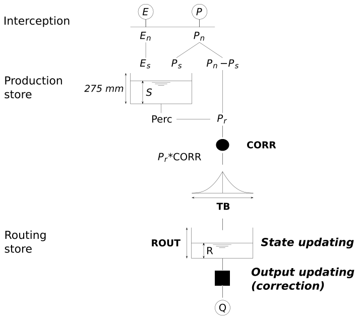
https://www.hydrol-earth-syst-sci.net/24/2017/2020/hess-24-2017-2020-f16

Figure A1The GRP model flow chart. After an interception step, the production function splits the net rainfall (P_n), according to the level of the production store. The effective rainfall (P_r) is the sum of the direct flow and the percolation from this store. A corrective multiplicative coefficient (CORR) is then applied. Then the flow runs through a unit hydrograph (time base: TB) and the routing store (capacity: ROUT).

Download

A snow module (Valéry et al., 2014) may be implemented on top of the model if necessary.

Like any GR model, it is parsimonious. It has only three parameters: (a) an adjustment factor of effective rainfall, which contributes to finding a good water balance; (b) the unit hydrograph time base used to account for the time lag between rainfall and streamflow; and (c) the capacity of the routing store, which temporally smooths the output signal.

Its main difference with the other GR models is the implementation “in the loop” of two data assimilation schemes:

a state-updating procedure which modifies the main state of the routing function as a function of the last discharge values,
output updating based on an autoregressive model of the multiplicative error or an artificial neural network (multi-layer perception) whose inputs are the last discharge value and the two last forecasting errors. In this study, the autoregressive model was used.

The parameters are calibrated in forecasting mode, i.e. with the application of the updating procedures. This model is used by the French flood forecasting services, some hydroelectricity suppliers and canal managers at an hourly time step in order to issue real-time forecasts for lead times ranging from a few hours to a few days at several hundred sites. Recently, Ficchì et al. (2016) paved the way to a multi-time-step GRP version.

Appendix B: The log–sinh transformation behaviours

B1 Log–sinh transformation formulations

In this study, we used the formulations of the log–sinh transformation chosen by Del Giudice et al. (2013):

\begin{matrix} (B1) & g_{3 [α, β]} : y \mapsto β \cdot \log (\sinh (\frac{α + y}{β})) . \end{matrix}

It is strictly equivalent to the formulation used by McInerney et al. (2017):

\begin{matrix} (B2) & g_{3 [a, b]}^{'} : y \mapsto \frac{1}{b} \log (\sinh (a + b \cdot y)) . \end{matrix}

B2 Different behaviours

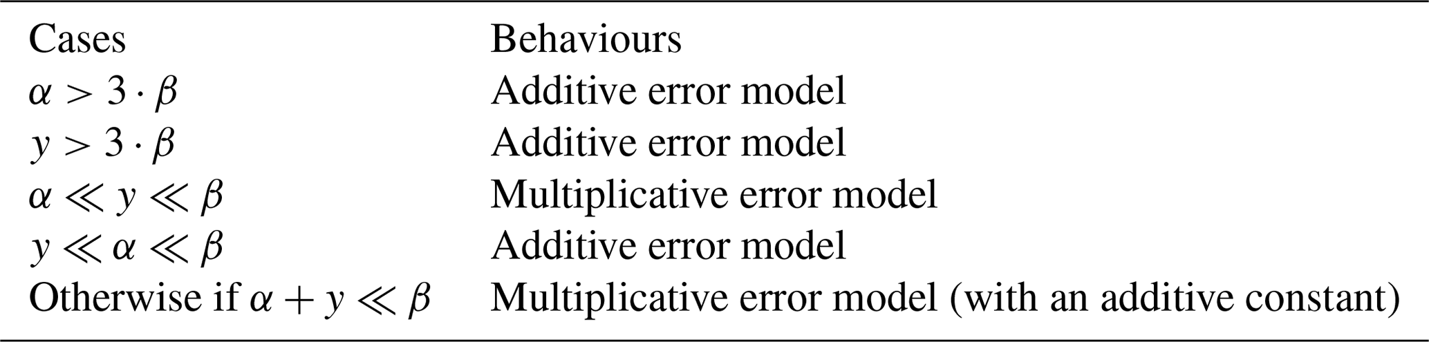
Depending on the relative values of α and β and on the value range of y, compared to α and β, the log–sinh transformation can be reduced to an affine transformation (i.e. $g_{3 [α, β]} (y + ε) - g_{3 [α, β]} (y) = δ \cdot ε$ ) or to the log transformation. The former case is equivalent to no transformation (identity function; additive error model), whereas the latter one is equivalent to a multiplicative error model (Table B1).

Table B1Summary of the different behaviours of the log–sinh transformation.

Download Print Version | Download XLSX

When y≪β,

\begin{array}{l} \sinh (\frac{α + y}{β}) & = \sinh (\frac{α}{β}) \cdot \cosh (\frac{y}{β}) \\ + \sinh (\frac{y}{β}) \cdot \cosh (\frac{α}{β}) \\ ≃ \sinh (\frac{α}{β}) \cdot (1 + \frac{y^{2}}{2 \cdot β^{2}} + \dots) \\ + \cosh (\frac{α}{β}) \cdot (\frac{y}{β} + \dots) . \end{array}

Thus,

g_{3 [α, β]} (y) ≃ β \cdot \log (\sinh (\frac{α}{β}) + \cosh (\frac{α}{β}) \cdot \frac{y}{β}) .

When α≪β, the latter results in

\begin{matrix} (B3) & g_{3 [α, β]} (y) ≃ β \cdot \log (\frac{α + y}{β}) . \end{matrix}

B2.1 Cases where the log–sinh transformation is equivalent to an affine transformation

If x>3 and $\sinh (x) \approx e^{x} / 2$ , then $\log (\sinh (x)) = x - \log (2)$ . Therefore when $z = (α + y) / β > 3$ , the log–sinh transformation is equivalent to an affine transformation. In such cases, $g_{3 [α, β]}^{- 1} (g_{3 [α, β]} (y) + ε) = y + ε$ .

This happens when

$α > 3 \cdot β$ ;
the β value is chosen to be large enough so that for any y value in the discharge range $y > 3 \cdot β$ .

Moreover, when $y ≪ α ≪ β$ , Eq. (B3) gives

\begin{array}{l} g_{3 [α, β]} & ≃ β \cdot [\log (\frac{α + y}{α}) + \log (α) - \log (β)] \\ ≃ \frac{β \cdot y}{α} + β \cdot (\log (α) - \log (β)) . \end{array}

The log–sinh transformation is then equivalent to an affine transformation.

B2.2 Cases where the log–sinh transformation is equivalent to a log transformation

As pointed out by McInerney et al. (2017), when $α ≪ y ≪ β$ , Eq. (B3) gives

g_{3 [α, β]} (y) ≃ β \cdot \log (\frac{y}{β}) .

The log–sinh transformation is then equivalent to a mere log transformation.

B3 Calibration

The α and β parameters are in the same physical dimension as the y variable. Since this study is dedicated to the extrapolation context, we used the following dimensionless parameterisation to calibrate the variable transformation in various catchments. α and β are compared to the maximum forecasted discharge in the D2_sup data subset:

\begin{matrix} (B4) & α = γ_{1} \cdot \max_{D 2} (\tilde{Q}) and β = γ_{2} \cdot \max_{D 2} (\tilde{Q}) . \end{matrix}

In the calibration step, the parameter space is explored on a (γ₁, γ₂) grid: 18 values of γ₁ from 0.01 to 100 and 15 values of γ₂ from 0.1 to 100 were tested, excluding combined values leading to the very same behaviours, such as $γ_{1} ≫ 3 \cdot γ_{2}$ , equivalent to no transformation (additive error model). A total of 200 (γ₁, γ₂) combinations were tested for each calibration.

Data availability

Data for this work were provided by Météo France (climatic data) and the hydrometric services of the French government (flow data). Readers can freely access streamflow observations used in this study at the Banque HYDRO website (http://www.hydro.eaufrance.fr/, last access: April 2020). Climate data can be retrieved on the Publithèque website of Météo France (https://publitheque.meteo.fr/, last access: April 2020). These data are not publicly available but can be provided for research and non-profit purposes – upon request to Météo France. Metadata on the catchments used in this study are detailed by Brigode et al. (2020) (https://doi.org/10.15454/UV01P1).

Supplement

The supplement related to this article is available online at: https://doi.org/10.5194/hess-24-2017-2020-supplement.

Author contributions

All co-authors contributed to the study and the article. LB and FB contributed equally and share co-first authorship.

Competing interests

The authors declare that they have no conflict of interest.

Acknowledgements

The authors thank the editor Dimitri Solomatine, Kolbjorn Engeland and one anonymous reviewer. Both reviewers provided insightful comments which helped to greatly improve this text. Thanks are also due to Météo-France for providing the meteorological data and Banque HYDRO database for the hydrological data. The contribution of the authors from Université Gustave Eiffel and INRAE was financially supported by SCHAPI (Ministry of the Environment).

Financial support

This research has been supported by SCHAPI (Ministry of the Environment) (grant nos. 21367400 (2018), 2201132931 (2018) and 2102615443 (2019)).

Review statement

This paper was edited by Dimitri Solomatine and reviewed by Kolbjorn Engeland and one anonymous referee.

References

Abaza, M., Anctil, F., Fortin, V., and Perreault, L.: On the incidence of meteorological and hydrological processors: Effect of resolution, sharpness and reliability of hydrological ensemble forecasts, J. Hydrol., 555, 371–384, https://doi.org/10.1016/j.jhydrol.2017.10.038, 2017. a

Abbaszadeh, P., Moradkhani, H., and Yan, H.: Enhancing hydrologic data assimilation by evolutionary Particle Filter and Markov Chain Monte Carlo, Adv, Water Resour,, 111, 192–204, https://doi.org/10.1016/j.advwatres.2017.11.011, 2018. a

Allamano, P., Laio, F., and Claps, P.: Effects of disregarding seasonality on the distribution of hydrological extremes, Hydrol. Earth Syst. Sci., 15, 3207–3215, https://doi.org/10.5194/hess-15-3207-2011, 2011. a

Anctil, F., Perrin, C., and Andréassian, V.: Impact of the length of observed records on the performance of ANN and of conceptual parsimonious rainfall-runoff forecasting models, Environ. Model. Softw., 19, 357–368, 2004. a

Andréassian, V., Hall, A., Chahinian, N., and Schaake, J.: Introduction and Synthesis: Why should hydrologists work on a large number of basin data sets?, IAHS-AISH Publication no. 307, International Association of Hydrological Sciences, Wallingford, UK, 1–5, 2006. a

Andréassian, V., Perrin, C., Berthet, L., Le Moine, N., Lerat, J., Loumagne, C., Oudin, L., Mathevet, T., Ramos, M.-H., and Valéry, A.: HESS Opinions “Crash tests for a standardized evaluation of hydrological models”, Hydrol. Earth Syst. Sci., 13, 1757–1764, https://doi.org/10.5194/hess-13-1757-2009, 2009. a

Andréassian, V., Le Moine, N., Perrin, C., Ramos, M.-H., Oudin, L., Mathevet, T., Lerat, J., and Berthet, L.: All that glitters is not gold: the case of calibrating hydrological models, Hydrol. Process., 26, 2206–2210, https://doi.org/10.1002/hyp.9264, 2012. a

Barbetta, S., Coccia, G., Moramarco, T., Brocca, L., and Todini, E.: The multi temporal/multi-model approach to predictive uncertainty assessment in real-time flood forecasting, J. Hydrol., 551, 555–576, https://doi.org/10.1016/j.jhydrol.2017.06.030, 2017. a, b

Bennett, J. C., Robertson, D. E., Shrestha, D. L., Wang, Q., Enever, D., Hapuarachchi, P., and Tuteja, N. K.: A System for Continuous Hydrological Ensemble Forecasting (SCHEF) to lead times of 9 days, J. Hydrol., 519, 2832–2846, https://doi.org/10.1016/j.jhydrol.2014.08.010, 2014. a

Berthet, L.: Flood forecasting at the hourly time-step: for a better assimilation of flow information in hydrological modelling, PhD thesis, Doctoral School GRN, AgroParisTech, Paris, Irstea, Antony, 2010. a

Berthet, L. and Piotte, O.: International survey for good practices in forecasting uncertainty assessment and communication, in: vol. 16, EGU General Assembly, April and May 2014, Vienna, Austria, EGU2014-8579, 2014. a

Berthet, L., Andréassian, V., Perrin, C., and Javelle, P.: How crucial is it to account for the antecedent moisture conditions in flood forecasting? Comparison of event-based and continuous approaches on 178 catchments, Hydrol. Earth Syst. Sci., 13, 819–831, https://doi.org/10.5194/hess-13-819-2009, 2009. a

Berthet, L., Andréassian, V., Perrin, C., and Loumagne, C.: How significant are quadratic criteria? Part 2. On the relative contribution of large flood events to the value of a quadratic criterion, Hydrolog. Sci. J., 55, 1063–1073, https://doi.org/10.1080/02626667.2010.505891, 2010. a

Bock, A. R., Farmer, W. H., and Hay, L. E.: Quantifying uncertainty in simulated streamflow and runoff from a continental-scale monthly water balance model, Adv. Water Resour., 122, 166–175, https://doi.org/10.1016/j.advwatres.2018.10.005, 2018. a

Bogner, K., Pappenberger, F., and Cloke, H. L.: Technical Note: The normal quantile transformation and its application in a flood forecasting system, Hydrol. Earth Syst. Sci., 16, 1085–1094, https://doi.org/10.5194/hess-16-1085-2012, 2012. a

Bourgin, F.: How to quantify predictive uncertainty in hydrological modelling? Exploratory work on a large sample of catchments, PhD thesis, Doctoral School GRNE, AgroParisTech, Paris, Irstea, Antony, 2014. a

Bourgin, F., Ramos, M., Thirel, G., and Andréassian, V.: Investigating the interactions between data assimilation and post-processing in hydrological ensemble forecasting, J. Hydrol., 519, 2775–2784, https://doi.org/10.1016/j.jhydrol.2014.07.054, 2014. a, b, c, d, e, f, g, h

Bourgin, F., Andréassian, V., Perrin, C., and Oudin, L.: Transferring global uncertainty estimates from gauged to ungauged catchments, Hydrol. Earth Syst. Sci., 19, 2535–2546, https://doi.org/10.5194/hess-19-2535-2015, 2015. a

Box, G. E. P. and Cox, D. R.: An Analysis of Transformations, J. Roy. Stat. Soc. B, 26, 211–252, 1964. a

Breiman, L.: Statistical modeling: The two cultures, Stat. Sci., 16, 199–215, https://doi.org/10.1214/ss/1009213726, 2001. a

Bremnes, J. B.: Constrained Quantile Regression Splines for Ensemble Postprocessing, Mon. Weather Rev., 147, 1769–1780, https://doi.org/10.1175/MWR-D-18-0420.1, 2019. a

Brigode, P., Oudin, L., and Perrin, C.: Hydrological model parameter instability: A source of additional uncertainty in estimating the hydrological impacts of climate change?, J. Hydrol., 476, 410–425, https://doi.org/10.1016/j.jhydrol.2012.11.012, 2013. a

Brigode, P., Génot, B., Lobligeois, F., Delaigue, O.: Summary sheets of watershed-scale hydroclimatic observed data for France, Portail Data INRAE, https://doi.org/10.15454/UV01P1, 2020. a

Buzzati, D.: Il deserto dei Tartari (The Tartar Steppe), Rizzoli, Milano, 1940. a

Cigizoglu, H.: Estimation, forecasting and extrapolation of river flows by artificial neural networks, Hydrolog. Sci. J., 48, 349–362, 2003. a

Coccia, G. and Todini, E.: Recent developments in predictive uncertainty assessment based on the model conditional processor approach, Hydrol. Earth Syst. Sci., 15, 3253–3274, https://doi.org/10.5194/hess-15-3253-2011, 2011. a, b

Coron, L., Andreassian, V., Perrin, C., Lerat, J., Vaze, J., Bourqui, M., and Hendrickx, F.: Crash testing hydrological models in contrasted climate conditions: An experiment on 216 Australian catchments, Water Resour. Res., 48, W05552, https://doi.org/10.1029/2011wr011721, 2012. a

Del Giudice, D., Honti, M., Scheidegger, A., Albert, C., Reichert, P., and Rieckermann, J.: Improving uncertainty estimation in urban hydrological modeling by statistically describing bias, Hydrol. Earth Syst. Sci., 17, 4209–4225, https://doi.org/10.5194/hess-17-4209-2013, 2013. a, b, c

Demargne, J., Wu, L., Regonda, S. K., Brown, J. D., Lee, H., He, M., Seo, D.-J., Hartman, R., Herr, H. D., Fresch, M., Schaake, J., and Zhu, Y.: The Science of NOAA's Operational Hydrologic Ensemble Forecast Service, B. Am. Meteorol. Soc., 95, 79–98, https://doi.org/10.1175/BAMS-D-12-00081.1, 2014. a, b

Demeritt, D., Cloke, H., Pappenberger, F., Thielen, J., Bartholmes, J., and Ramos, M.-H.: Ensemble predictions and perceptions of risk, uncertainty, and error in flood forecasting, Environ. Hazards, 7, 115–127, 2007. a

Dogulu, N., López López, P., Solomatine, D. P., Weerts, A. H., and Shrestha, D. L.: Estimation of predictive hydrologic uncertainty using the quantile regression and UNEEC methods and their comparison on contrasting catchments, Hydrol. Earth Syst. Sci., 19, 3181–3201, https://doi.org/10.5194/hess-19-3181-2015, 2015. a

Ficchì, A., Perrin, C., and Andréassian, V.: Impact of temporal resolution of inputs on hydrological model performance: An analysis based on 2400 flood events, J. Hydrol., 538, 454–470, https://doi.org/10.1016/j.jhydrol.2016.04.016, 2016. a, b

Furusho, C., Perrin, C., Viatgé, J., R., L., and Andréassian, V.: Collaborative work between operational forecasters and scientists for better flood forecasts, La Houille Blanche, 2016-4, 5–10, https://doi.org/10.1051/lhb/2016033, 2016. a

Gaume, E., Bain, V., Bernardara, P., Newinger, O., Barbuc, M., Bateman, A., Blaskovicová, L., Blöschl, G., Borga, M., Dumitrescu, A., Daliakopoulos, I., Garcia, J., Irimescu, A., Kohnova, S., Koutroulis, A., Marchi, L., Matreata, S., Medina, V., Preciso, E., Sempere-Torres, D., Stancalie, G., Szolgay, J., Tsanis, I., Velasco, D., and Viglione, A.: A compilation of data on European flash floods, J. Hydrol., 367, 70–78, https://doi.org/10.1016/j.jhydrol.2008.12.028, 2009. a

Giustolisi, O. and Laucelli, D.: Improving generalization of artificial neural networks in rainfall-runoff modelling, Hydrolog. Sci. J., 50, 439–457, 2005. a

Gneiting, T., Balabdaoui, F., and Raftery, A. E.: Probabilistic forecasts, calibration and sharpness, J. Roy. Stat. Soc. B, 69, 243–268, https://doi.org/10.1111/j.1467-9868.2007.00587.x, 2007. a, b

Gupta, H. V., Perrin, C., Blöschl, G., Montanari, A., Kumar, R., Clark, M., and Andréassian, V.: Large-sample hydrology: a need to balance depth with breadth, Hydrol. Earth Syst. Sci., 18, 463–477, https://doi.org/10.5194/hess-18-463-2014, 2014. a

Hemri, S., Lisniak, D., and Klein, B.: Multivariate postprocessing techniques for probabilistic hydrological forecasting, Water Resour. Res., 51, 7436–7451, https://doi.org/10.1002/2014WR016473, 2015. a, b

Hersbach, H.: Decomposition of the continuous ranked probability score for ensemble prediction systems, Weather Forecast., 15, 559–570, https://doi.org/10.1175/1520-0434(2000)015<0559:dotcrp>2.0.co;2, 2000. a, b

Imrie, C., Durucan, S., and Korre, A.: River flow prediction using artificial neural networks: Generalisation beyond the calibration range, J. Hydrol., 233, 138–153, 2000. a

Kelly, K. S. and Krzysztofowicz, R.: A bivariate meta-Gaussian density for use in hydrology, Stoch. Hydrol. Hydraul., 11, 17–31, 1997. a

Klemes̆, V.: Operational testing of hydrological simulation models, Hydrolog. Sci. J. – Journal Des Sciences Hydrologiques, 31, 13–24, https://doi.org/10.1080/02626668609491024, 1986. a, b

Krzysztofowicz, R.: Bayesian theory of probabilistic forecasting via deterministic hydrologic model, Water Resour. Res., 35, 2739–2750, 1999. a, b, c

Krzysztofowicz, R. and Maranzano, C. J.: Hydrologic uncertainty processor for probabilistic stage transition forecasting, J. Hydro., 293, 57–73, https://doi.org/10.1016/j.jhydrol.2004.01.003, 2004. a

Laio, F. and Tamea, S.: Verification tools for probabilistic forecasts of continuous hydrological variables, Hydrol. Earth Syst. Sci., 11, 1267–1277, https://doi.org/10.5194/hess-11-1267-2007, 2007. a

Lang, M., Pobanz, K., Renard, B., Renouf, E., and Sauquet, E.: Extrapolation of rating curves by hydraulic modelling, with application to flood frequency analysis, Hydrolog. Sci. J., 55, 883–898, https://doi.org/10.1080/02626667.2010.504186, 2010. a

Legates, D. and McCabe Jr., G.: Evaluating the use of `goodness-of-fit' measures in hydrologic and hydroclimatic model validation, Water Resour. Res., 35, 233–241, 1999. a

Leleu, I., Tonnelier, I., Puechberty, R., Gouin, P., Viquendi, I., Cobos, L., Foray, A., Baillon, M., and Ndima, P.-O.: Re-founding the national information system designed to manage and give access to hydrometric data, La Houille Blanche, 2014-1, 25–32, https://doi.org/10.1051/lhb/2014004, 2014. a

Li, M., Wang, Q. J., and Bennett, J.: Accounting for seasonal dependence in hydrological model errors and prediction uncertainty, Water Resour. Res., 49, 5913–5929, https://doi.org/10.1002/wrcr.20445, 2013. a

Li, W., Duan, Q., Miao, C., Ye, A., Gong, W., and Di, Z.: A review on statistical postprocessing methods for hydrometeorological ensemble forecasting, Wiley Interdisciplin. Rev.: Water, 4, e1246, https://doi.org/10.1002/wat2.1246, 2017. a, b

Liano, K.: Robust error measure for supervised neural network learning with outliers, IEEE T. Neural Netw., 7, 246–250, 1996. a

Lobligeois, F., Andréassian, V., Perrin, C., Tabary, P., and Loumagne, C.: When does higher spatial resolution rainfall information improve streamflow simulation? An evaluation using 3620 flood events, Hydrol. Earth Syst. Sci., 18, 575–594, https://doi.org/10.5194/hess-18-575-2014, 2014. a

McInerney, D., Thyer, M., Kavetski, D., Lerat, J., and Kuczera, G.: Improving probabilistic prediction of daily streamflow by identifying Pareto optimal approaches for modeling heteroscedastic residual errors, Water Resour. Res., 53, 2199–2239, https://doi.org/10.1002/2016WR019168, 2017. a, b, c, d, e, f

Merz, R., Parajka, J., and Blöschl, G.: Time stability of catchment model parameters: Implications for climate impact analyses, Water Resour. Res., 47, W02531, https://doi.org/10.1029/2010WR009505, 2011. a

Michel, C.: Que peut-on faire en hydrologie avec un modèle conceptuel à un seul paramètre?, La Houille Blanche, 1983-1, 39–44, https://doi.org/10.1051/lhb/1983004, 1983. a

Montanari, A.: Uncertainty of Hydrological Predictions, in: Treatise on Water Science, edited by: Wilderer, P., Elsevier, Oxford, 459–478, 2011. a

Montanari, A. and Grossi, G.: Estimating the uncertainty of hydrological forecasts: A statistical approach, Water Resour. Res., 44, W00B08, https://doi.org/10.1029/2008wr006897, 2008. a

Moradkhani, H., Hsu, K. L., Gupta, H., and Sorooshian, S.: Uncertainty assessment of hydrologic model states and parameters: Sequential data assimilation using the particle filter, Water Resour. Res., 41, W05012, https://doi.org/10.1029/2004wr003604, 2005a. a

Moradkhani, H., Sorooshian, S., Gupta, H. V., and Houser, P. R.: Dual state–parameter estimation of hydrological models using ensemble Kalman filter, Adv. Water Resour., 28, 135–147, https://doi.org/10.1016/j.advwatres.2004.09.002, 2005b. a

Morawietz, M., Xu, C.-Y., Gottschalk, L., and Tallaksen, L. M.: Systematic evaluation of autoregressive error models as post-processors for a probabilistic streamflow forecast system, J. Hydrol., 407, 58–72, https://doi.org/10.1016/j.jhydrol.2011.07.007, 2011. a, b

Oudin, L., Hervieu, F., Michel, C., Perrin, C., Andreassian, V., Anctil, F., and Loumagne, C.: Which potential evapotranspiration input for a lumped rainfall-runoff model? Part 2 – Towards a simple and efficient potential evapotranspiration model for rainfall-runoff modelling, J. Hydrol., 303, 290–306, https://doi.org/10.1016/j.jhydrol.2004.08.026, 2005. a

Pagano, T. C., Shrestha, D. L., Wang, Q. J., Robertson, D., and Hapuarachchi, P.: Ensemble dressing for hydrological applications, Hydrol. Process., 27, 106–116, https://doi.org/10.1002/hyp.9313, 2013. a

Pagano, T. C., Wood, A. W., Ramos, M.-H., Cloke, H. L., Pappenberger, F., Clark, M. P., Cranston, M., Kavetski, D., Mathevet, T., Sorooshian, S., and Verkade, J. S.: Challenges of Operational River Forecasting, J. Hydrometeorol., 15, 1692–1707, https://doi.org/10.1175/JHM-D-13-0188.1, 2014. a

Pappenberger, F. and Beven, K. J.: Ignorance is bliss: Or seven reasons not to use uncertainty analysis, Water Resour. Res., 42, W05302, https://doi.org/10.1029/2005wr004820, 2006. a

Pappenberger, F., Thielen, J., and Del Medico, M.: The impact of weather forecast improvements on large scale hydrology: analysing a decade of forecasts of the European Flood Alert System, Hydrol. Process., 25, 1091–1113, https://doi.org/10.1002/hyp.7772, 2011. a

Pappenberger, F., Pagano, T. C., Brown, J. D., Alfieri, L., Lavers, D. A., Berthet, L., Bressand, F., Cloke, H. L., Cranston, M., Danhelka, J., Demargne, J., Demuth, N., de Saint-Aubin, C., Feikema, P. M., Fresch, M. A., Garçon, R., Gelfan, A., He, Y., Hu, Y. Z., Janet, B., Jurdy, N., Javelle, P., Kuchment, L., Laborda, Y., Langsholt, E., Le Lay, M., Li, Z. J., Mannessiez, F., Marchandise, A., Marty, R., Meißner, D., Manful, D., Organde, D., Pourret, V., Rademacher, S., Ramos, M. H., Reinbold, D., Tibaldi, S., Silvano, P., Salamon, P., Shin, D., Sorbet, C., Sprokkereef, E., Thiemig, V., Tuteja, N. K., van Andel, S. J., Verkade, J. S., Vehviläinen, B., Vogelbacher, A., Wetterhall, F., Zappa, M., Van der Zwan, R. E., and Thielen-del Pozo, J.: Hydrological Ensemble Prediction Systems Around the Globe, Springer, Berlin, Heidelberg, 1–35, https://doi.org/10.1007/978-3-642-40457-3_47-1, 2016. a

Perrin, C., Michel, C., and Andreassian, V.: Improvement of a parsimonious model for streamflow simulation, J. Hydrol., 279, 275–289, https://doi.org/10.1016/s0022-1694(03)00225-7, 2003. a

Perrin, C., Oudin, L., Andréassian, V., Rojas-Serna, C., Michel, C., and Mathevet, T.: Impact of limited streamflow data on the efficiency and the parameters of rainfall-runoff models, Hydrolog. Sci. J., 52, 131–151, 2007. a

Ramos, M.-H., Bartholmes, J., and Pozo, J. T.-D.: Development of decision support products based on ensemble forecasts in the European flood alert system, Atmos. Sci. Lette., 8, 113–119, https://doi.org/10.1002/asl.161, 2007. a

Reichert, P. and Mieleitner, J.: Analyzing input and structural uncertainty of nonlinear dynamic models with stochastic, time-dependent parameters, Water Resour. Res., 45, W10402, https://doi.org/10.1029/2009wr007814, 2009. a

Renard, B., Kavetski, D., Kuczera, G., Thyer, M., and Franks, S. W.: Understanding predictive uncertainty in hydrologic modeling: The challenge of identifying input and structural errors, Water Resour. Res., 46, W05521, https://doi.org/10.1029/2009wr008328, 2010. a, b, c, d

Salamon, P. and Feyen, L.: Assessing parameter, precipitation, and predictive uncertainty in a distributed hydrological model using sequential data assimilation with the particle filter, J. Hydrol., 376, 428–442, https://doi.org/10.1016/j.jhydrol.2009.07.051, 2009. a, b

Schoups, G. and Vrugt, J. A.: A formal likelihood function for parameter and predictive inference of hydrologic models with correlated, heteroscedastic, and non-Gaussian errors, Water Resour. Res., 46, W10531, https://doi.org/10.1029/2009wr008933, 2010. a, b

Seiller, G., Anctil, F., and Roy, R.: Design and experimentation of an empirical multistructure framework for accurate, sharp and reliable hydrological ensembles, J. Hydrol., 552, 313–340, https://doi.org/10.1016/j.jhydrol.2017.07.002, 2017. a

Sharma, S., Siddique, R., Reed, S., Ahnert, P., Mendoza, P., and Mejia, A.: Relative effects of statistical preprocessing and postprocessing on a regional hydrological ensemble prediction system, Hydrol. Earth Syst. Sci., 22, 1831–1849, https://doi.org/10.5194/hess-22-1831-2018, 2018. a

Singh, S. K., McMillan, H., and Bardossy, A.: Use of the data depth function to differentiate between case of interpolation and extrapolation in hydrological model prediction, J. Hydrol., 477, 213–228, https://doi.org/10.1016/j.jhydrol.2012.11.034, 2013. a, b

Solomatine, D. P. and Shrestha, D. L.: A novel method to estimate model uncertainty using machine learning techniques, Water Resour. Res., 45, W00B11, https://doi.org/10.1029/2008wr006839, 2009. a

Tabary, P., Dupuy, P., L'Henaff, G., Gueguen, C., Moulin, L., Laurantin, O., Merlier, C., and Soubeyroux, J.-M.: A 10-year (1997–2006) reanalysis of Quantitative Precipitation Estimation over France: methodology and first results, in: vol. 351, IAHS, Wallingford, UK, 255–260, 2012. a

Thielen, J., Bartholmes, J., Ramos, M.-H., and de Roo, A.: The European Flood Alert System – Part 1: Concept and development, Hydrol. Earth Syst. Sci., 13, 125–140, https://doi.org/10.5194/hess-13-125-2009, 2009. a

Todini, E.: Role and treatment of uncertainty in real-time flood forecasting, Hydrol. Process., 18, 2743–2746, https://doi.org/10.1002/hyp.5687, 2004. a

Todini, E.: Hydrological catchment modelling: past, present and future, Hydrol. Earth Syst. Sci., 11, 468–482, https://doi.org/10.5194/hess-11-468-2007, 2007. a, b

Todini, E.: A model conditional processor to assess predictive uncertainty in flood forecasting, Int. J. River Basin Manage., 6, 123–137, https://doi.org/10.1080/15715124.2008.9635342, 2008. a

Todini, E.: Predictive uncertainty assessment in real time flood forecasting, in: Uncertainties in Environmental Modelling and Consequences for Policy Making, edited by: Baveye, P. C., Laba, M., and Mysiak, J., Springer Netherlands, Dordrecht, 205–228, 2009. a

Valéry, A., Andréassian, V., and Perrin, C.: `As simple as possible but not simpler': What is useful in a temperature-based snow-accounting routine? Part 2 – Sensitivity analysis of the Cemaneige snow accounting routine on 380 catchments, J. Hydrol., 517, 1176–1187, https://doi.org/10.1016/j.jhydrol.2014.04.058, 2014. a

Van Steenbergen, N., Ronsyn, J., and Willems, P.: A non-parametric data-based approach for probabilistic flood forecasting in support of uncertainty communication, Environ. Model. Softw., 33, 92–105, https://doi.org/10.1016/j.envsoft.2012.01.013, 2012. a

Vaze, J., Post, D., Chiew, F., Perraud, J.-M., Viney, N., and Teng, J.: Climate non-stationarity – Validity of calibrated rainfall–runoff models for use in climate change studies, J. Hydrol., 394, 447–457, https://doi.org/10.1016/j.jhydrol.2010.09.018, 2010. a

Velazquez, J. A., Anctil, F., and Perrin, C.: Performance and reliability of multimodel hydrological ensemble simulations based on seventeen lumped models and a thousand catchments, Hydrol. Earth Syst. Sci., 14, 2303–2317, https://doi.org/10.5194/hess-14-2303-2010, 2010. a

Verkade, J. S. and Werner, M. G. F.: Estimating the benefits of single value and probability forecasting for flood warning, Hydrol. Earth Syst. Sci., 15, 3751–3765, https://doi.org/10.5194/hess-15-3751-2011, 2011. a

Verkade, J. S., Brown, J., Davids, F., Reggiani, P., and Weerts, A.: Estimating predictive hydrological uncertainty by dressing deterministic and ensemble forecasts; a comparison, with application to Meuse and Rhine, J. Hydrol., 555, 257–277, https://doi.org/10.1016/j.jhydrol.2017.10.024, 2017. a

Viatgé, J., Pinna, T., Perrin, C., Dorchies, D., and Garandeau, L.: Towards an enhanced temporal flexibility of the GRP flood forecasting operational model, in: Proceedings of the SHF conference “De la prévision des crues à la gestion de crise” (From flood forecasting to crisis management), 14–16 November 2018, Société Hydrotechnique de France, Avignon, France, p. 12, 2018. a

Viatgé, J., Berthet, L., Marty, R., Bourgin, F., Piotte, O., Ramos, M. H., and Perrin, C.: Towards the real-time production of predictive intervals around streamflow forecasts in Vigicrues in France, La Houille Blanche, 2019-1, 63–71, https://doi.org/10.1051/lhb/2019016, 2019. a

Wang, Q. J., Robertson, D. E., and Chiew, F. H. S.: A Bayesian joint probability modeling approach for seasonal forecasting of streamflows at multiple sites, Water Resour. Res., 45, W05407, https://doi.org/10.1029/2008wr007355, 2009. a, b

Wang, Q. J., Shrestha, D. L., Robertson, D. E., and Pokhrel, P.: A log-sinh transformation for data normalization and variance stabilization, Water Resour. Res., 48, W05514, https://doi.org/10.1029/2011wr010973, 2012. a

Wani, O., Beckers, J. V. L., Weerts, A. H., and Solomatine, D. P.: Residual uncertainty estimation using instance-based learning with applications to hydrologic forecasting, Hydrol. Earth Syst. Sci., 21, 4021–4036, https://doi.org/10.5194/hess-21-4021-2017, 2017. a

Weerts, A. H., Winsemius, H. C., and Verkade, J. S.: Estimation of predictive hydrological uncertainty using quantile regression: examples from the National Flood Forecasting System (England and Wales), Hydrol. Earth Syst. Sci., 15, 255–265, https://doi.org/10.5194/hess-15-255-2011, 2011. a, b

Wilby, R. L.: Uncertainty in water resource model parameters used for climate change impact assessment, Hydrol. Process., 19, 3201–3219, https://doi.org/10.1002/hyp.5819, 2005. a

Woldemeskel, F., McInerney, D., Lerat, J., Thyer, M., Kavetski, D., Shin, D., Tuteja, N., and Kuczera, G.: Evaluating post-processing approaches for monthly and seasonal streamflow forecasts, Hydrol. Earth Syst. Sci., 22, 6257–6278, https://doi.org/10.5194/hess-22-6257-2018, 2018. a

Wright, D. P., Thyer, M., and Westra, S.: Influential point detection diagnostics in the context of hydrological model calibration, J. Hydrol., 527, 1161–1172, https://doi.org/10.1016/j.jhydrol.2015.05.047, 2015. a

Yang, J., Reichert, P., and Abbaspour, K. C.: Bayesian uncertainty analysis in distributed hydrologic modeling: a case study in the Thur River basin (Switzerland), Water Resour. Res., 43, W10401, https://doi.org/10.1029/2006wr005497, 2007a. a

Yang, J., Reichert, P., Abbaspour, K. C., and Yang, H.: Hydrological modelling of the Chaohe Basin in China: Statistical model formulation and Bayesian inference, J. Hydrol., 340, 167–182, https://doi.org/10.1016/j.jhydrol.2007.03.006, 2007b. a, b, c

Zalachori, I., Ramos, M. H., Garçon, R., Mathevet, T., and Gailhard, J.: Statistical processing of forecasts for hydrological ensemble prediction: a comparative study of different bias correction strategies, Adv. Sci. Res., 8, 135–141, https://doi.org/10.5194/asr-8-135-2012, 2012. a

Articles

Short summary

An increasing number of flood forecasting services assess and communicate the uncertainty associated with their forecasts. We present a crash-testing framework that evaluates the quality of hydrological forecasts in an extrapolation context. Overall, the results highlight the challenge of uncertainty quantification when forecasting high flows. They show a significant drop in reliability when forecasting high flows and considerable variability among catchments and across lead times.

A crash-testing framework for predictive uncertainty assessment when forecasting high flows in an extrapolation context

1.1 The big one: dream or nightmare for the forecaster?

1.2 Obtaining reliable forecasts remains a challenging task

1.2.1 Modelling each source of uncertainty

1.2.2 Post-processing approaches

1.2.3 Combining different approaches

1.3 Scope

2.1 Data and forecasting model

2.1.1 Catchments and hydrological data

2.1.2 Hydrological model

2.1.3 Empirical hydrological uncertainty processor (EHUP)

2.1.4 The different transformation families

2.2 Methodology: a testing framework designed for extrapolation context assessment

2.2.1 Testing framework

2.2.2 Events selection

2.2.3 Selection of the data subsets

2.2.4 Calibration and evaluation steps

2.3 Performance criteria and calibration

2.3.1 Probabilistic evaluation framework

2.3.2 The calibration criterion

3.1 Results with the calibration data set D2sup

3.2 Results with the D3 control data set

3.2.1 Reliability

3.2.2 Other performance metrics

3.3 Investigating the performance loss in an extrapolation context

4.1 Do more complex parametric transformations yield better results in an extrapolation context?

4.2 Empirically based versus distribution-based approaches: does the distribution shape choice impact the uncertainty assessment in an extrapolation context?

4.3 A need for a focus change?

5.1 Main findings

5.2 Limitations and perspectives

B1 Log–sinh transformation formulations

B2 Different behaviours

B2.1 Cases where the log–sinh transformation is equivalent to an affine transformation

B2.2 Cases where the log–sinh transformation is equivalent to a log transformation

B3 Calibration

3.1 Results with the calibration data set D2_sup