the Creative Commons Attribution 4.0 License.
the Creative Commons Attribution 4.0 License.
 | 23 Apr 2020
A methodology to estimate flow duration curves at partially ungauged basins
Elena Ridolfi
Hemendra Kumar
András Bárdossy
The flow duration curve (FDC) of streamflow at a specific site has a key role in the knowledge on the distribution and characteristics of streamflow at that site. The FDC gives information on the water regime, providing information to optimally manage the water resources of the river. In spite of its importance, because of the lack of streamflow gauging stations, the FDC construction can be a not straightforward task. In partially gauged basins, FDCs are usually built using regionalization among the other methods. In this paper we show that the FDC is not a characteristic of the basin only, but of both the basin and the weather. Different weather conditions lead to different FDCs for the same catchment. The differences can often be significant. Similarly, the FDC built at a site for a specific period cannot be used to retrieve the FDC at a different site for the same time window. In this paper, we propose a new methodology to estimate FDCs at partially gauged basins (i.e., target sites) using precipitation data gauged at another basin (i.e., donor site). The main idea is that it is possible to retrieve the FDC of a target period of time using the data gauged during a given donor time period for which data are available at both target and donor sites. To test the methodology, several donor and target time periods are analyzed and results are shown for different sites in the USA. The comparison between estimated and actually observed FDCs shows the reasonability of the approach, especially for intermediate percentiles.


A duration curve is a function that associates with a specific variable its exceedance frequency. Specifically, in hydrology a flow duration curve (FDC) is a function describing the flow variability at a specific site during a period of interest. It represents the streamflow values, gauged at a site, against their relative probability of exceedance. An empirical long-term FDC is the complement of the empirical cumulative distribution function of streamflow values at a given time resolution based on the complete streamflow record available for the basin of interest (Castellarin et al., 2007). FDCs are built as explained in the following:
-
rank the streamflow values in descending order;
-
plot the sorted values against their corresponding frequency of exceedance.
The duration di of the ith sorted observation is its exceedance probability Pi. If Pi is estimated using a Weibull plotting position (Weibull, 1939), the duration di for any qi (with i=1; …; N) is
where N is the length of the streamflow series and qi is the ith sorted streamflow value.
The FDC provides historical information on the water regime. Several time resolutions of streamflow data can be used to build the FDC: annual, monthly or daily. However, the finer the resolution is, the higher the information provided by the FDC is about the hydrological characteristics of the river (Smakhtin, 2001). FDCs may be built either on the basis of the whole available record period (Vogel, 1994), on the basis of all similar months (Smakhtin et al., 1997), or on the basis of a specific month.
In one curve, the FDC condenses a wealth of hydrologic information that can be easily accessed. Because of the key role of runoff variability in both water resource management and environmental health maintenance, the FDC is used in a large variety of applications as reported by Vogel (1994). For instance, the FDC can quantify the capacity of the river to meet intake requests as it provides information about the reliability of the water resource for water abstraction activities (Dingman, 1981). It is at the base of hydropower plants' design as they are used to determine the hydropower energy potential, especially for run-of-river plants (Hänggi and Weingartner, 2012; Blöschl et al., 2013). As the FDC is a key signature of runoff variability, it can be used to assess the impact of changes in a catchment. To this end, through the FDC, Vogel et al. (2007) introduced the indicators of the eco-deficit and eco-surplus. Moreover, the FDC can be used to define and investigate low flows (Smakhtin, 2001). The knowledge of the streamflow characteristics is also relevant for stream water quality studies, for instance, to regulate the proper threshold for chemical concentration and load (Bonta and Cleland, 2003). The FDC has a further application in model calibration. This application is based on the replication of the flow frequency distribution rather than of the simulation of the hydrograph (Yu and Yang, 2000; Westerberg et al., 2011). Other applications are related to irrigation planning (Chow, 1964); schedule optimal flow release from reservoirs (Alaouze, 1991); basin afforestation (Scott et al., 2000); investigation of the effects on the flow regime due to basin vegetation change (Brown et al., 2005).
In spite of its importance, the FDC is affected by the lack of data in ungauged and poorly gauged basins. Many authors dealt with the issue of FDC prediction at ungauged or partially gauged locations through regional regression (e.g., Fennessey and Vogel, 1990; Mohamoud, 2008; Rianna et al., 2011, 2013; Castellarin et al., 2013; Pugliese et al., 2016) and geostatistical interpolation (e.g., Pugliese et al., 2014). Ganora et al. (2009) developed a methodology to estimate FDC at ungauged sites based on distance measures that can be related to the catchment and the climatic characteristics. Spatial nonlinear interpolation methods were developed by several scholars (e.g., Archfield and Vogel, 2010; Mohamoud, 2008; Hughes and Smakhtin, 1996; Farmer et al., 2014). Worland et al. (2019) presented a method involving the use of the copula function. Hughes and Smakhtin (1996) proposed a method to extend and/or fill in daily flow time series at a site using monthly FDCs of the target site itself. These monthly FDCs should be recorded during a donor period or retrieved using different methods such as (i) regionalization of FDCs based on available observed records from several adjacent gauges (Smakhtin et al., 1997) or (ii) conversion of FDCs calculated from monthly data into 1 d FDCs (Smakhtin, 1999). Since the main limitation of the approach proposed by Hughes and Smakhtin (1996) is that it is based entirely on observed flow records, later, Smakhtin and Masse (2000) proposed a further development, which uses the current precipitation index (CPI) of the donor site to extend the daily hydrograph at the target site. The major assumption is that both the CPIs occurring at donor sites in a reasonably close proximity to the target site and target site's flows themselves correspond to similar percentage points on their respective duration curves. On the other hand, the basic assumption of the spatial interpolation algorithm proposed by Hughes and Smakhtin (1996) is that flows occurring simultaneously at sites in reasonably close proximity to each other correspond to similar probabilities on their respective flow duration curves. In contrast, one important message of our paper is that FDCs can be very different from time period to time period, both at the site itself and at pairs of sites as a long-term change in the weather affects the FDCs. Therefore, our approach is based on the concept that proximal sites do not share similar FDCs. This will be demonstrated in the paper by applying a two-sample Kolmogorov–Smirnov test to pairs of stations. The usual assumption that they and the related indices are characteristic for the basin is not true. Therefore, the FDCs built at a given location for different periods cannot be regarded as the same distribution. It is not possible to determine a unique distribution and therefore a unique set of parameters. The same results from the analysis of FDCs built in two different basins. It is not possible to develop relations between parameters of the basin and characteristics of the FDC to yield synthesized FDCs in locations where flow data are not available, as done for instance by Quimpo et al. (1983). These issues have a key role especially when dealing with ungauged basins.
The main idea underlying our work is to build the FDC at a target site using a filter, which relates the distributions of the discharge and the precipitation. As the weather is the main driver of annual runoff variability, we propose a transformation driven by the weather. The paper is organized as follows. First, the case study is presented and basins are grouped into energy- and water-limited ones. Then, the Kolmogorov–Smirnov test is carried out on pairs of FDCs to assess whether these curves can be regarded as the same distribution. Second, the methodology is presented together with the underlying assumptions. Then, the approach is applied to a set of basins located in the case study area. Finally, results are shown and discussed.
Table 1US case study area: streamflow gauges and corresponding basin characteristics.
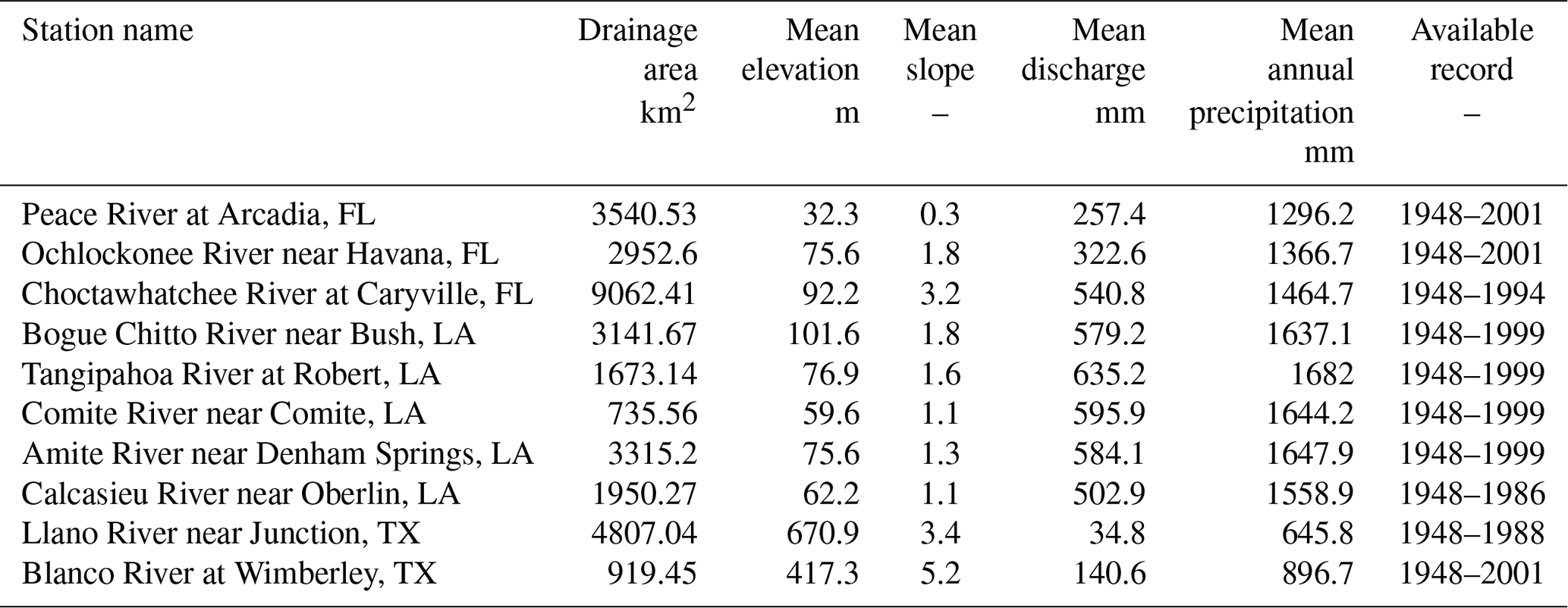
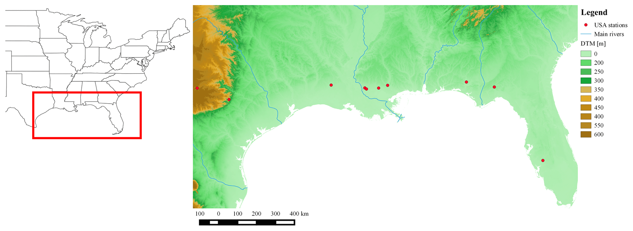
Figure 1Streamflow gauges (red circles) used to test the methodology in the corresponding US basins. DTM retrieved from Jarvis et al. (2008).
The methodology was applied to several basins located in three different states on the Gulf coast of the USA: Florida, Louisiana and Texas (Fig. 1). These basins were selected because they are characterized by a mild climate and, therefore, no snow events have been recorded, allowing us to neglect the snow melting effect. Daily streamflow discharge and precipitation values are available for each basin for different time windows (Table 1).
Daily streamflow discharge data were originally provided by the United States Geological Survey (USGS) gauges, while mean areal precipitation and climatic potential evaporation were supplied by the National Centers for Environmental Information, formerly the National Climate Data Center (NCDC) at daily resolution. The data set is a subset of the Model Parameter Estimation Experiment (MOPEX) database, used for hydrological model comparison studies (Duan et al., 2006) and for simultaneous calibration of hydrological models (Bárdossy et al., 2016).
2.1 Energy- and water-limited basins
Annual runoff variability is driven by the relative availability of water (i.e., precipitation) and energy (i.e., evaporation potential). Therefore, the weather is the most important driver of annual variability (Blöschl et al., 2013). Much of the annual runoff variability can be explained by observing the different availability of water and energy. For instance, if more water arrives at the basin than energy can remove through evaporation, the annual runoff will be high. Moreover, in this case the relationship between runoff and precipitation will be more linear than when more energy is available to evaporate the water. On the other hand, in an arid region, the aridity of the climate determines a high inter-annual runoff variability because of the nonlinear relationship between runoff and precipitation. Therefore, differences in water and energy availability cause differences in annual runoff variability. However, additional factors such as differences in seasonality and precipitation must be considered (Jothityangkoonad and Sivapalan, 2009). The relative availability of water and energy can be described through the Budyko curve (Budyko, 1974). The curve plots the ratio between mean annual actual evaporation and mean annual precipitation as a function of the ratio between mean annual potential evaporation and mean annual precipitation. Therefore, it defines a similarity index (i.e., the aridity index) to express the availability of water and energy and thus bolsters the classification of hydrological sceneries into various degrees of aridity. The Budyko curve represents the effects of water and energy availability on annual runoff variability. Moreover, it provides an indication of the synchrony of evaporation and precipitation. For instance, where precipitation and evaporation are in phase, runoff production declines since the basin allows for infiltration and stores water and vice versa. Many regions range from in phase to out of phase because of the strong seasonality of climate forcing. However, the climatic timing can influence runoff variability as presented by Montanari et al. (2006). In this framework, it is important to understand the behavior of the basins under analysis. To this end, we analyzed the mean annual runoff coefficient, the annual precipitation and the annual evapotranspiration against the annual mean temperature. This analysis is essential to understand the causal processes leading to the long-term mean and variability of runoff as also described in McMahon et al. (2013). The mean annual runoff coefficient is defined as
where is the annual discharge volume and is the annual precipitation volume.
Results show that basins have two different behaviors: precipitation, evapotranspiration and runoff have either a positive or a negative correlation with the air temperature. In the former case the evapotranspiration is limited by the available water, which happens in water-limited basins; in the latter the evapotranspiration is limited by the available energy, which happens in energy-limited basins. For instance, measurements at Peace River (LA) suggest that the basin is balanced between energy and water limitation by the correlation criterion (Fig. 2 upper panel), while Ochlockonee River (FL), Amite River near Denham Springs (LA) and Bogue Chitto River (LA) are energy-limited. Results for Amite River are consistent with what was found by Carrillo et al. (2011). Since it is not possible to infer discharge values of a water-limited basin from the data set of an energy-limited one, analyses have been carried out on climatically homogeneous sets of basins.
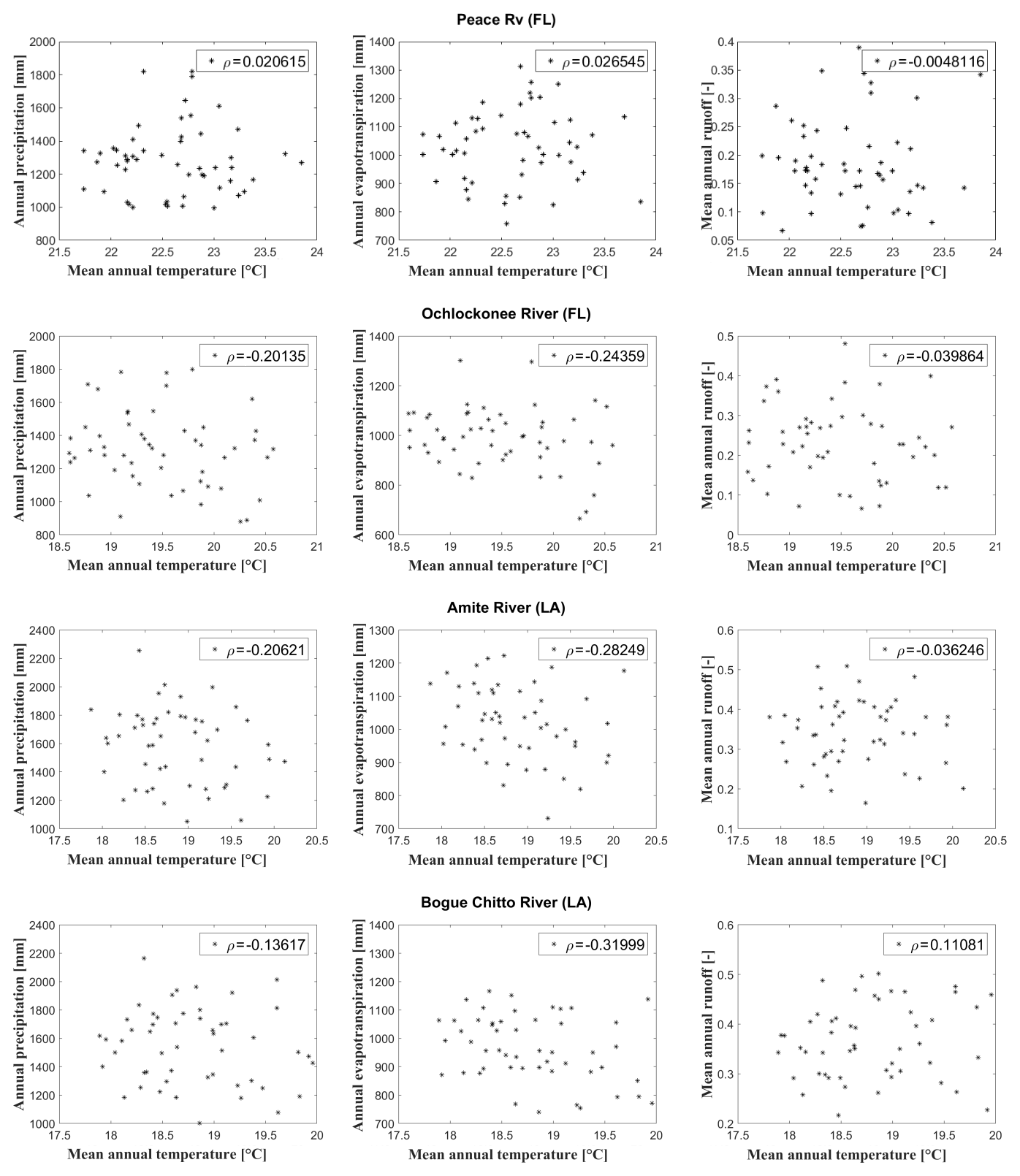
Figure 2Annual precipitation against mean annual temperature (left panels), annual evapotranspiration against mean annual temperature (middle panels) and annual runoff coefficient against mean annual temperature (right panels) for four different basins: Peace River (FL), Ochlockonee River (FL), Amite River near Denham Springs (LA), and Bogue Chitto River (LA). In each plot, the Pearson correlation coefficient ρ is reported in the box.
2.2 Preliminary analysis
The FDC can be interpreted as a distribution function of discharge over a given time period. To determine whether samples are drawn from the same distribution, here the two-sample Kolomogorov–Smirnov test (KS; Massey, 1951) is carried out on each pair of samples. The KS statistic on two samples is a non-parametric test for the null hypothesis that the two independent samples are drawn from the same continuous distribution. The decision to reject the null hypothesis is based on comparing the p value with the significance level set equal to 5 %. Moreover, the test allows us to estimate the distance between couples of FDC:
where F1(x) is the proportion of x1 values less than or equal to x and F2(x) is the proportion of x2 values less than or equal to x. F1 and F2 are two FDCs. The KS statistic is applied to daily streamflow data sampled in several periods of record (e.g., 1 year, 10 years, 15 years). The long memory is relatively low, and we consider full years; thus, annual cycles do not have an influence on our results. The test is carried out both on pairs of samples gauged at the same location in two different years (or in two different decades) and on pairs sampled at two different sites. Since the streamflow data present autocorrelation, the autocorrelation affects the KS test. Weiss (1978) proposed a methodology to account for modifying the KS test for autocorrelated data. Later, Xu (2014) suggested a method that can be applied to a two-sample test. The information contained in the data is (usually) less than an independent and identically distributed (i.i.d.) sample with the same size. In other words, the number of equivalent independent observations is less than the sample size. In the following, we explain how we accounted for the equivalent sample size. It is easier to implement and, more importantly, it can be easily generalized to a two-sample test. We can assume that the autocorrelation effect attenuates after 3 d. For instance, let us take as an example a 1-year FDC. If the sample was 3 times smaller and for instance the length would equal 122 (i.e., 365 divided by 3), the null hypothesis would have been rejected anyway, leading to the same conclusion (i.e., the two samples cannot be regarded as the same distribution). This is due to the fact that, according to the two-sample KS test, the length of the equivalent sample that could pass the test should be 22.
The application of the KS test to our samples is pivotal to the development of the methodology. Test results show that streamflow data gauged in different periods (e.g., years or decades) at a specific location do not have the same distribution. The consequence is that it is not possible to use the parameters and the distribution derived from a FDC built for a specific time window to build the FDC of another time window. The same results comparing streamflow data were gauged in a specific year or decade at two different sites. Since the two data sets cannot be regarded as the same distribution, it is not possible to derive the FDC at one location using the parameters of the FDC sampled at another location. Therefore, it is necessary to develop a methodology that accounts for the weather, as it is the main driver of FDC variability as shown in the following. Figure 3 shows the magnitude of the difference between FDCs built at the same location using streamflow data gauged during different time windows.
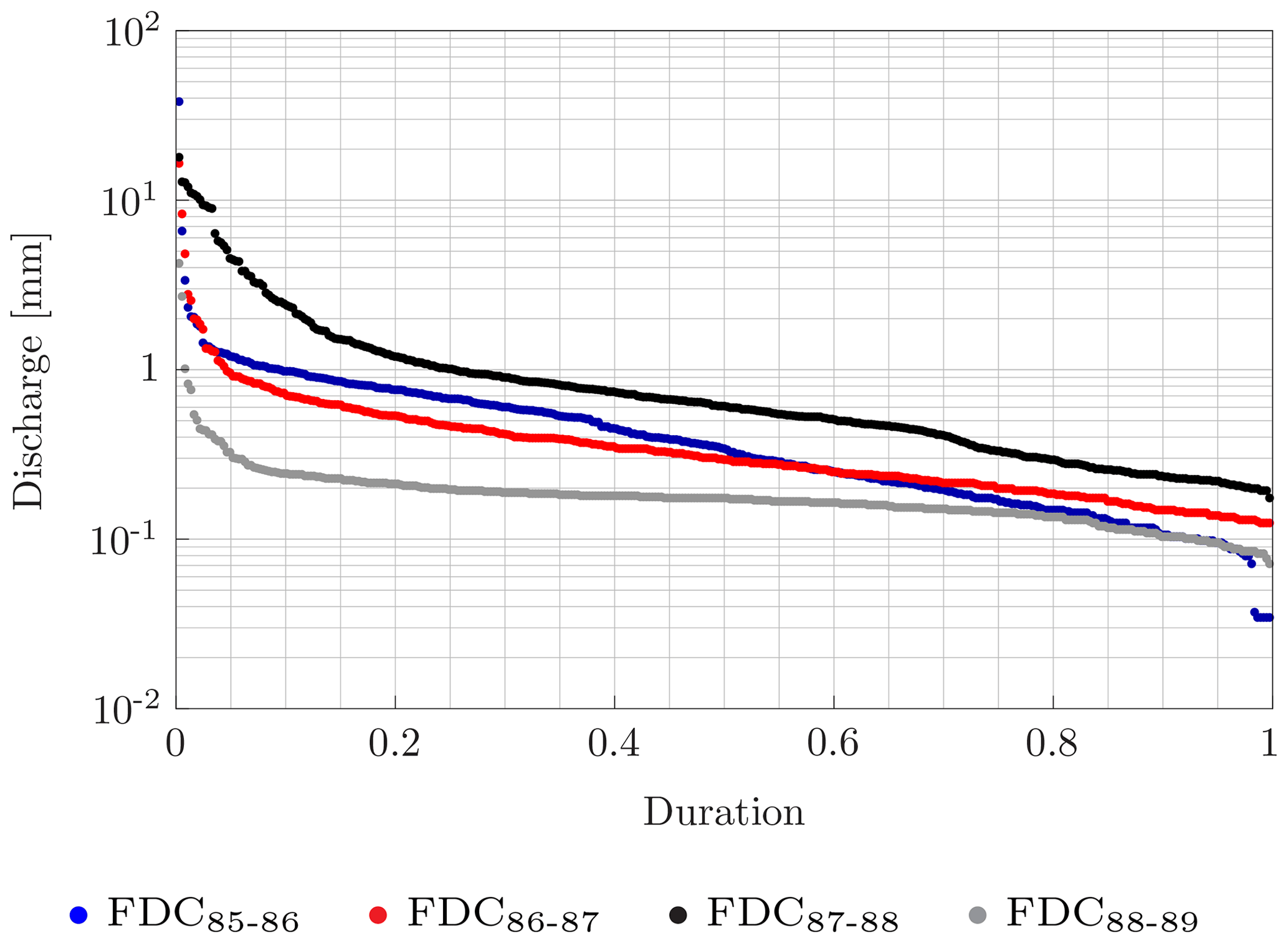
Figure 3FDCs built for Tangipahoa River (FL) for four different hydrological years. Every hydrological year starts in October and ends the following September.
The aim of this paper is to find the distribution of Qk(t) for a time period (T1, T2), that is, a FDC. We assume that discharge is related to precipitation in the form
where k is a generic site, hk is the transformation, usually approximated by a hydrological model, Pk is the precipitation and βk is the specific parameter of the hydrological model. The core of this work is to retrieve the discharge values without hydrological modeling as modeling often introduces additional errors and may be biased for long subperiods. Thus, the main idea is to get rid of a complicated nonlinear process and to find a filter which relates the distributions.
The main hypothesis underlying this work is that daily flow duration curves at a partially ungauged location can be found with knowledge of the precipitation record at a donor site. The most important descriptor of the weather characteristic is the rainfall; however, we cannot use the distribution of Pk to assess the FDC directly as it will fail due to the lacking temporal structure and the many zeros. We can then use a transformation of Pk, the Antecedent Precipitation Index (API):
Both transformations reported in Eqs. (4) and (5) can be regarded as filters acting on Pk. These filters do not necessarily produce highly correlated series, but may produce series with similar distributions. The API is used to investigate precipitation data in a similar way to discharge data as it combines in a streamflow-like way the history of the precipitation. It represents the memory of a basin as it is related to the amount of water released by the soil to the river considering a given time window. Specifically, the API allows us to take into account the antecedent conditions and the duration of the rainfall events and gives an estimate of the portion of rainfall contributing to storm runoff (Linsley et al., 1949). It is a sequence of linear combinations of rainfall events in the period preceding a specific storm (Kohler and Linsley, 1951). For a resolution of 1 d and a time window of 30 d, the API at the ith day is given by
where α is a constant and ranges from 0 to 1 and Pi is the daily precipitation that occurred on the ith day (Kohler and Linsley, 1951). When α tends to zero, API keeps tracks of the precipitation that occurred on the few previous days, and it represents the short memory of the basin. When α tends to 1, the API represents the long memory of the basin as it includes the effect of precipitation that occurred many days before. To capture the latter behavior, in this study α is chosen equal to 0.85. This is in agreement with a previous study by Sugimoto et al. (2016), who investigated a case study area whereby a preliminary analysis was performed (i.e., Neckar basin); nevertheless, this value was found to be suitable also for the US basins. Here the API is calculated from areal precipitation instead of point precipitation.
Formally the basic hypotheses of this paper are the following.
-
Flow duration curves are not invariant properties of basins, but are the product of basin, weather and human interactions. In this investigation we do not consider the human interactions.
-
Precipitation is the most important influencing factor on discharge.
-
Basins delay the reaction on precipitation; therefore, the API is a better indicator of the influence of precipitation on discharge.
-
We assume that discharge and API are changing in a similar way for longer time periods.
Let be the distribution of daily discharges at basin A and time period Ti (flow duration curve for the selected time period) and be the distribution of daily API at basin A and time period Ti.
The transformation from Ti to Tj provides an estimated :
This is a quantile–quantile transformation.
The basic question can be written in the form of the following equation:
That can be summarized in the following question: do the percentiles of the API change in the same way as those of the discharge? Note that if the relationship between API and discharge is a good one-to-one relationship, then the two sides are nearly equal. Even a weak relationship can do a good job if the errors are independent and the signal of the change is correct. Figures 4 and 5 show the difference between the real change in percentiles and that obtained by using the API for different time periods according to Eq. (9). Note that the assumption that the FDC is time-invariant would imply that the lines for the discharge are on the diagonal.
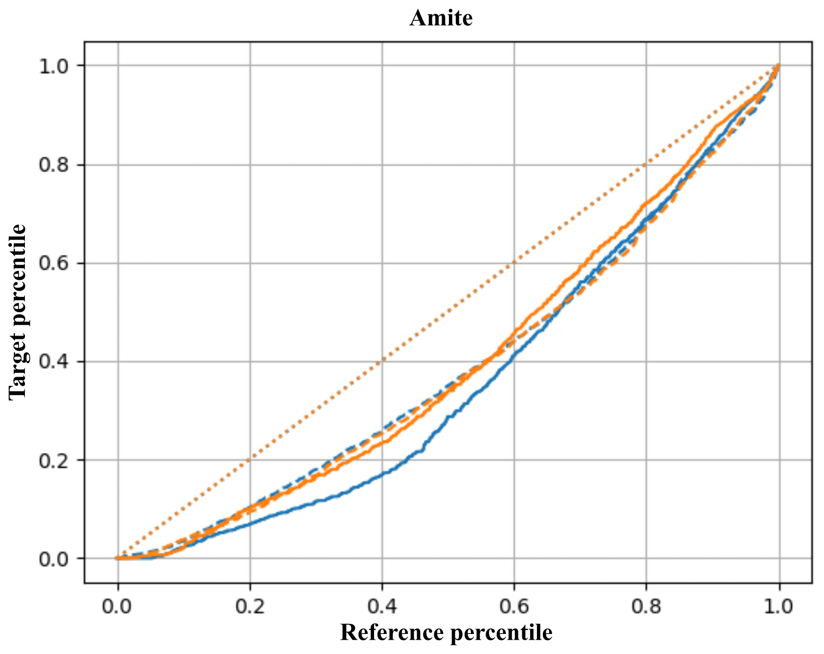
Figure 4The transformation functions of the 1951–1960 FDC (solid) and API (dashed) to the target periods 1971–1980 (blue) and 1981–1990 (orange) for Amite. For the sake of comparison, the diagonal is dotted in orange.
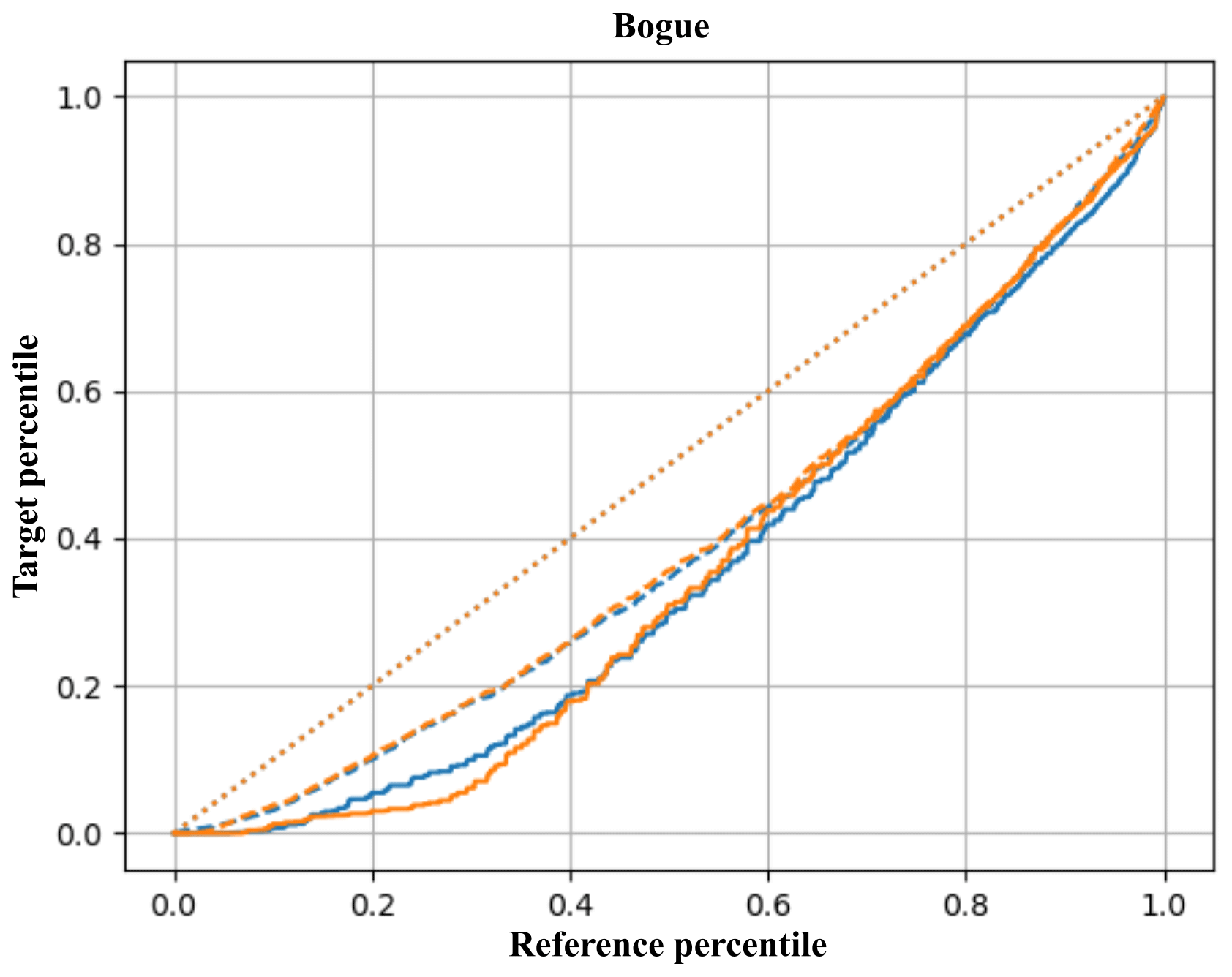
Figure 5The transformation functions of the 1951–1960 FDC (solid) and API (dashed) to the target periods 1971–1980 (blue) and 1981–1990 (orange) for Bogue. For the sake of comparison, the diagonal is dotted in orange.
The correlation between API and discharge is around 0.6, but the transformations are quite similar and the API-based transformation delivers good FDCs.
If the API is changing continuously in space, then one can use the change in the FDC of a different location B for the estimation:
In the following, the methodology is reported step by step; then, the performance criteria used to estimate the goodness of the methodology are presented.
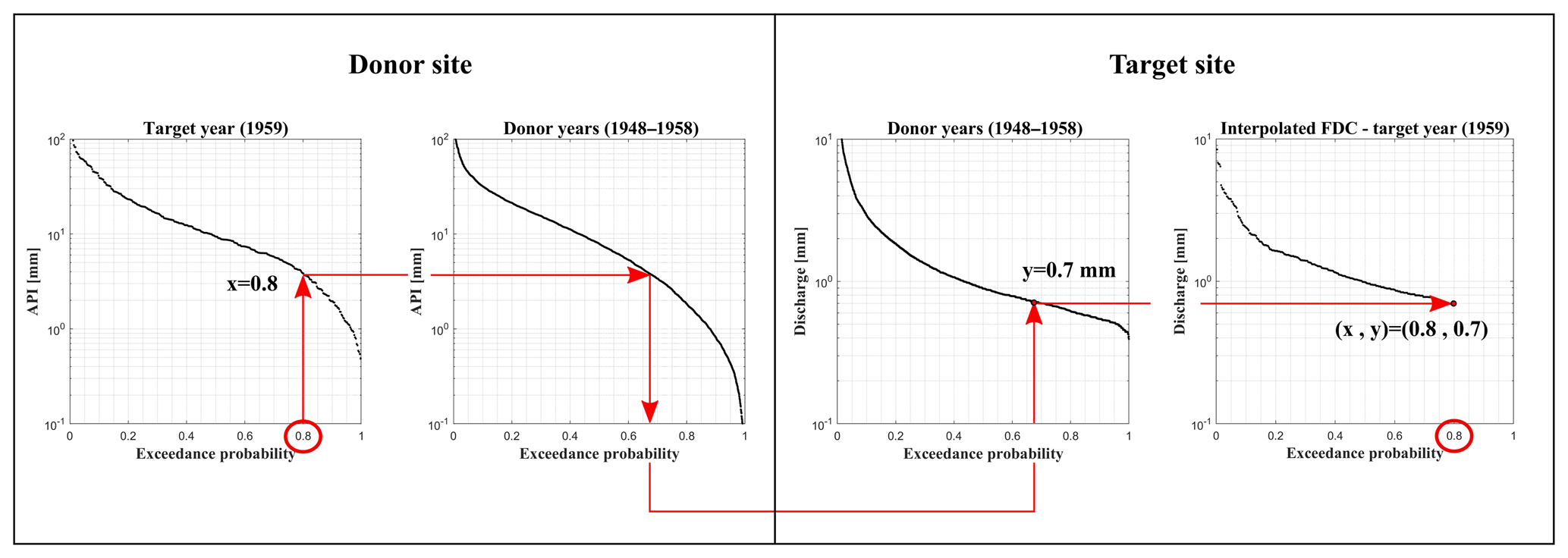
Figure 6Illustration of FDC generation using the interpolation with the API of the donor site as a proxy.
3.1 Procedure step by step
Let us consider two basins, A and B. We want to determine the flow duration curve at basin B from data available at A. Therefore, A is the donor basin, while B is the target basin. Let us suppose that in a given number of years, discharge is available at site B, named donor years, while they are not available for another number of years, i.e., the target years. Precipitation is available at A for both donor and target years.
-
Donor year selection. Select a number of years for which precipitation and discharge values are available at daily resolution for basins A and B, respectively. These will be named donor years (e.g., with durations of 1 year, 10, 15, or 20 years).
-
Estimation of the exceedance probability of API values. For site A for donor and target years, sort API values in descending order and assign to each sorted value the corresponding rank and estimate the corresponding frequency of exceedance using the Weibull plotting position.
-
Estimation of the exceedance probability of streamflow values. Exceedance probability of streamflow values are calculated for site B for donor years only.
-
Data transfer from donor site.
- i.
Select the ith probability pi, with i=1, …, Nt, where Nt is the length of the target sample and the corresponding API value recorded at the donor site during the target years (Fig. 6a).
- ii.
Search for this API value among those recorded at the donor site during the donor years and estimate the corresponding exceedance probability (Fig. 6b).
- iii.
This probability is then used to retrieve the corresponding streamflow value recorded at site B during the donor years (Fig. 6c).
- iv.
This streamflow value is the missing value at site B corresponding to the ith exceedance probability pi (Fig. 6d).
- i.
Steps from 1 to 4 are repeated for every exceedance probability and then for different target periods and target basins. The FDC is expressed in millimeters; thus, the area of the basin is not an issue using data of another basin.
An example of the procedure is reported step by step in Appendix A.
3.2 Performance criteria
To determine the performance of the procedure proposed in this paper, different criteria are selected: the Nash–Sutcliffe efficiency index (NSE; Nash and Sutcliffe, 1970), the BIAS and the mean absolute error (MAE).
The Nash–Sutcliffe efficiency between the interpolated and observed flow values is the most widespread performance criterion:
where Qobs is the observed discharge value at the target basin during the target period; is the mean value of the observed discharge during the target period in the target basin; Qintrpl is the interpolated discharge value.
The BIAS represents the mean difference between observed and interpolated values (Castellarin et al., 2001; Ridolfi et al., 2016):
This metric comprises the mean of the error made relative to the observed record. It is a signed and unbounded metric. It indicates as a ratio the level of overall agreement between the observed and interpolated values.
The mean absolute error is defined as
Discharge values are in millimeters and so is the MAE. It measures the overall agreement between observed and interpolated values. It is a non-negative metric without upper or lower bounds. A perfect model would result in a MAE equal to zero. This estimation metric does not provide any information about under- or over-estimation, but it determines all deviations from the observed values regardless of the sign. All metrics are evaluated here for a specific set of percentiles; thus, N is the number of discharge values related to a specific ith percentile. In binning by percentiles, all percentages were rounded down to the nearest whole number.
The procedure explained above was tested on several target basins varying both donor and target periods.

Figure 7Interpolated FDC at Tangipahoa River (FL) and Bogue River (LA), in the upper and lower panels, respectively. The donor basin is Blanco River (TX). The donor years are a 20-year time window from October 1948 to September 1968 and from October 1968 to September 1988. Target years are the decades shown above each panel. Blue and red dots are the observed and interpolated FDC at the target basin during the target period, respectively; the black dots are the observed FDC at the donor basin during the target period. In each box the Kolmogorov–Smirnov distance between observed and interpolated values, D*, is reported. The p value of the test is always around zero, but for Tangipahoa target years 1948–1958.
Results show a good agreement between observed and interpolated FDCs. For instance, the FDCs interpolated using 20 and 10 years as donor and target periods, respectively, have a good performance, as shown for Tangipahoa and Bogue basins (Fig. 7). The method performance is higher for intermediate durations, while it can be lower for the low flows, e.g., as at Bogue for target years 1988–1998 (Fig. 7, lower panels) and for the high flows. The good performance of the approach is also noticeable when the target period is 15 years (Fig. 8). In each panel, the two-sample Kolmogorov–Smirnov test distance between observed and interpolated values, D*, is reported. D* is characterized by small values showing a good performance of the method. Since usually the FDC of a donor site is used to retrieve the FDC of a target site for the same period, the FDC of the donor basin recorded during the target period is also plotted. It is noteworthy to observe that the difference between these two FDCs can be substantial. This implies that the FDCs can be substantially different at different sites in the same period of time.
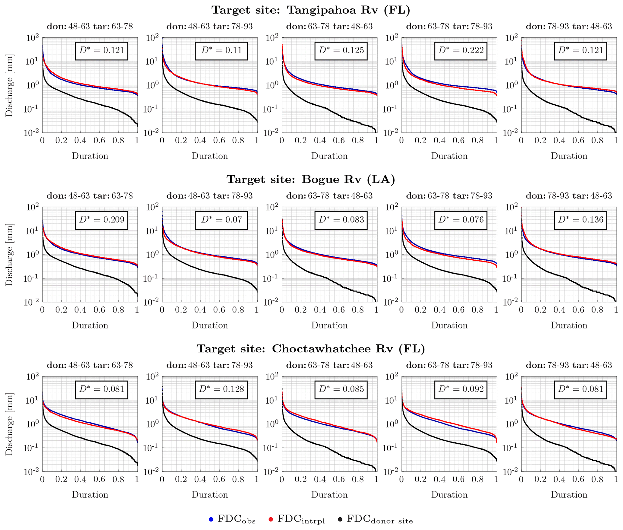
Figure 8Interpolated FDC at Tangipahoa River (FL), Bogue River (LA) and Choctawhatchee River (FL), in the upper, middle and lower panels, respectively. The donor basin is Blanco River (TX). The donor and target years are periods of 15 years. The blue and red dots are observed and interpolated FDC, respectively, at the target basin during the target period; the black dots are the observed FDC at the donor basin during the target period. In each box the KS distance, D*, is reported. The p value of D* is always around zero.
Interpolated and observed FDCs almost perfectly match when obtained using long donor and target periods (Figs. 7 and 8). On the other hand, when the target period is short, the performance decreases, as also shown by the KS distance, D*, reported in each single panel of Fig. 9 where the target period equals 1 year. As a matter of fact, the donor period being constant, the KS distance is much higher when the target period is 1 year (Fig. 9) and the p value of the test is always zero, but for hydrologic years 1972–1973 and 1976–1977. Nevertheless, the interpolated and observed FDCs have a high agreement in shape, as for instance at Tangipahoa River for all but one (i.e., 1969–1970) target year. In these cases, the difference between the two curves could be due to the different temperature values characterizing the donor and target basins. This affects the evapotranspiration in the two basins and, therefore, the streamflow values.
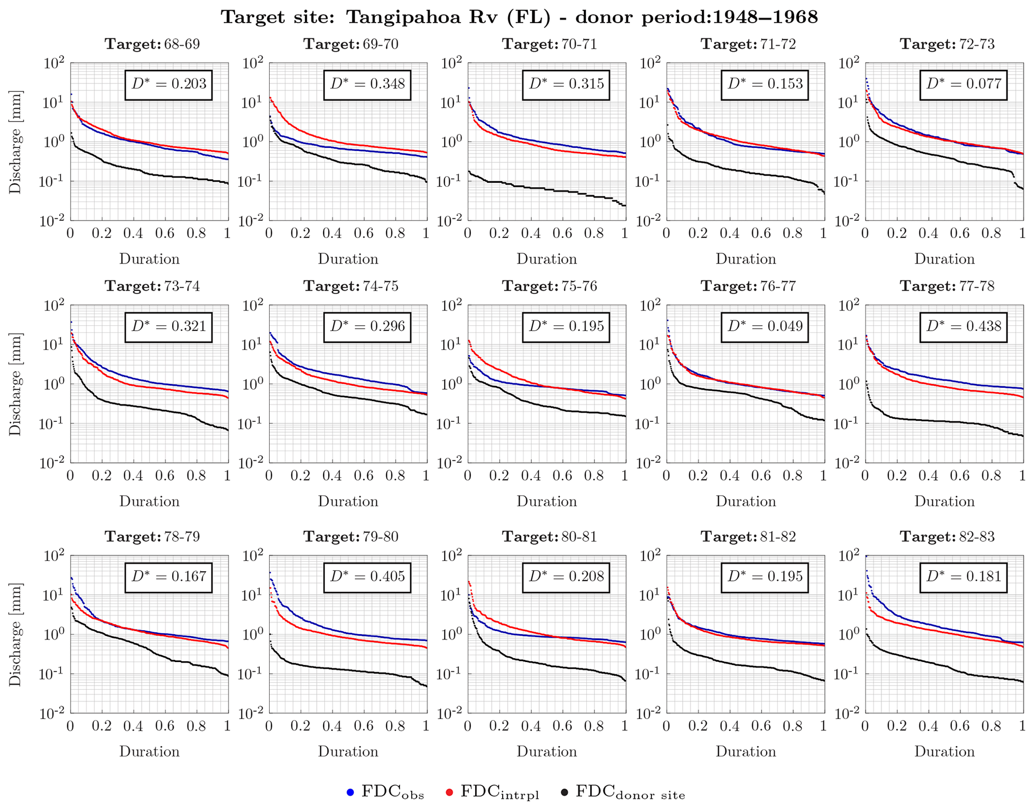
Figure 9Interpolated FDC at Tangipahoa River (FL). The donor basin is Blanco River (TX). The donor years are a 20-year time window from October 1948 to September 1968. Target years are each hydrological year from October 1968 to September 1983. The blue and red dots are observed and interpolated FDC, respectively, at the target basin during the target period; the black dots are the observed FDC at the donor basin during the target period. In each box the Kolmogorov–Smirnov distance, D*, is reported. The p value of the test is always around zero, but for hydrologic years 1972–1973 and 1976–1977.
Results suggest that the API gives effectively a good estimation of the memory of the basin and can be used to represent the precipitation similarly to the discharge.
To estimate the goodness of the methodology, the NSE, BIAS and MAE are evaluated for the 1st, 3rd, 5th, 10th, 20th, 30th, 50th, 75th, 90th and 99th percentiles.
When a decade is used as both target and donor period, the performance measures show a good agreement between observed and interpolated values (Fig. 10). The NSE index shows accurate estimation; i.e., it is characterized by values close to 1, especially of intermediate percentiles. The BIAS provides information regarding the overall agreement between interpolated and observed values. Its magnitude is likely higher for high flows, while it attenuates for intermediate percentiles. The MAE also shows a low performance for high streamflow values. This is due to the fact that the procedure is more able to reproduce the average streamflow values than extreme events such as high and low flows. However, low flows are more likely well estimated rather than high flows.
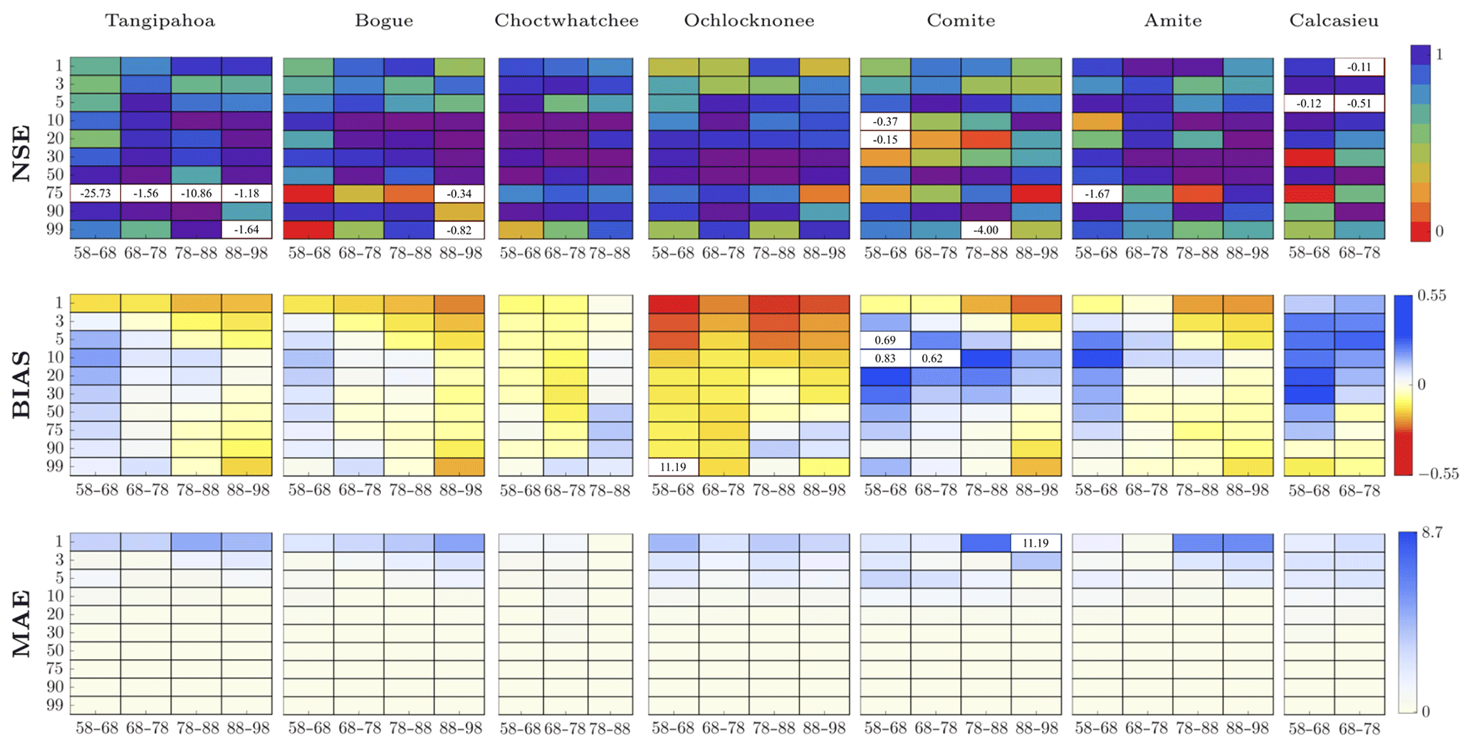
Figure 10Performance measures NSE, BIAS and MAE evaluated for specific percentiles (on the y axis) and for specific target decades on the x axis. The donor decade is 1948–1958 and the donor basin is Blanco (TX). Each target basin is indicated in the corresponding box. Negative values of the NSE as well as outliers of BIAS and MAE are reported in the corresponding box.
When both target and donor periods equal 15 years, the agreement between interpolated and observed flow values is high (Fig. 11). The NSE shows values of efficiency around 1; thus, there is a good match between interpolated and observed values, even though there are a few exceptions. The errors are very low in value, as shown by the MAE, which also reveals a poor performance for high flows, while the performance improves for intermediate and low flows. The high flows are more likely estimated with a higher error than intermediate and low flows, as also shown by the BIAS.
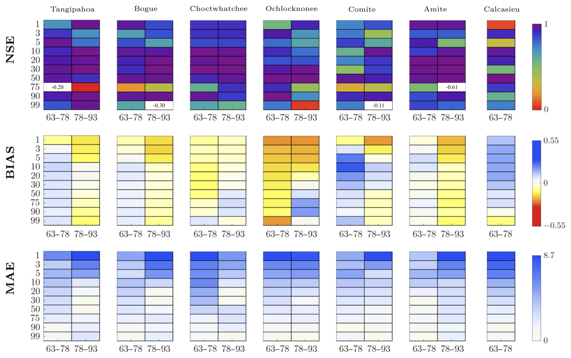
Figure 11Performance measures NSE, BIAS and MAE evaluated for specific percentiles (on the y axis) and for specific 15 target years (i.e., 1963–1978 and 1978–1993 on the x axis). The donor decade is 1948–1963 and the donor basin is Blanco (TX). Each target basin is indicated in the corresponding box. Negative values of the NSE are reported in the corresponding box.
As resulted from the KS test applied to pairs of FDCs obtained from recorded data at the same site in different periods, FDCs cannot be considered an invariant characteristic of a basin. The fact that FDCs are not invariant suggests that the weather is a driver of annual runoff variability. Indeed, the reason should be found in the weather conditions, as others (e.g., the basin area, the land use) did not change. To better investigate these findings, we performed the KS test on pairs of observed and interpolated FDCs for two purposes. The first is to know whether pairs of interpolated and observed FDCs at the same site have the same continuous distribution; the second is to know which is the distance between these pairs. The test performed on pairs of interpolated and observed FDCs revealed that the null hypothesis could not be rejected for nearly half of the cases. For instance, for Tangipahoa River the test was not rejected in 48 % of the cases (Fig. 12b). On the contrary, the test rejected the null hypothesis that FDCs built at the same location in different periods had the same distribution. In 73 % of the cases, the distance between pairs of interpolated and observed FDCs of the same period is smaller than the distance between FDCs built at the same site from data recorded during different periods (Fig. 12b and a, respectively). These results suggest that the methodology proposed here has a good performance, and it is actually an interesting alternative to other methodologies, which assume that FDCs of different periods have the same distribution.
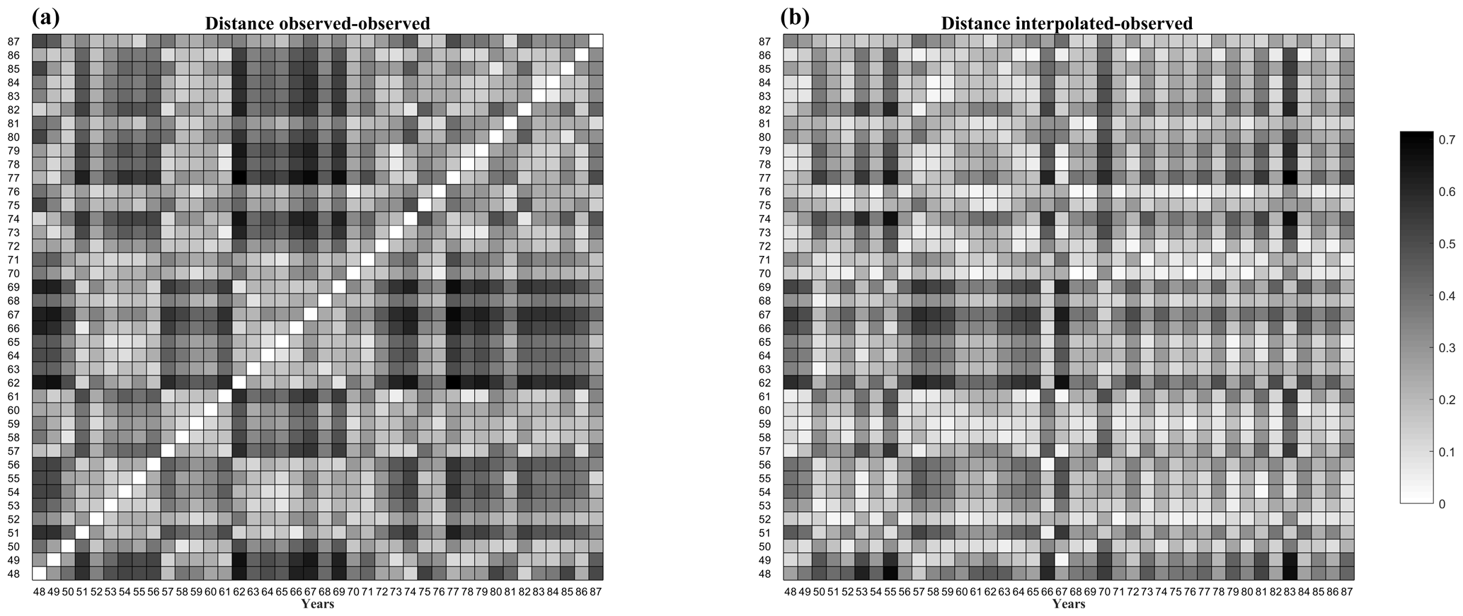
Figure 12Kolmogorov–Smirnov distance between couples of streamflow values observed (a) and between couples of streamflow values observed and interpolated (b) at Tangipahoa River (FL) from October 1948 to September 1987.
As the weather conditions strongly influence the FDC estimation, we analyzed the streamflow percentiles to assess the between-year variability. To this end, the moving average (MA) of the 30th, 70th, 90th and 95th percentiles of streamflow is estimated. The MA values are estimated using three different fixed time windows (i.e., 10, 15 and 20 years; Fig. 13).
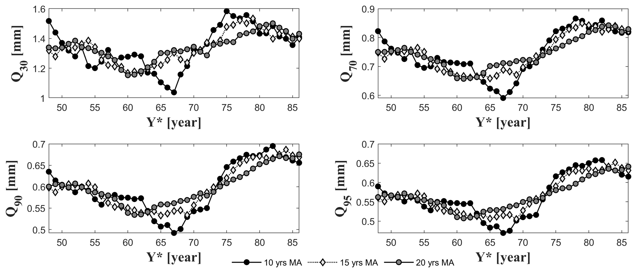
Figure 13Moving average (MA) of the 30th, 70th, 90th and 95th percentiles of daily streamflow values gauged at Tangipahoa. Three different fixed time windows are used to estimate the MA: 10, 15 and 20 years. On the x axis the first year of each interval is plotted (Y*).
It is interesting to observe that the MA values are characterized by a strong variability throughout the time. The fluctuation of the flow percentiles suggests that the percentiles cannot be considered an invariant characteristic of the basin. Therefore, it is not possible to estimate the flow quantiles using regression methods that do not consider the weather characteristics. These methods, first, regionalize empirical runoff percentiles using multiple regression models. Then, regional evaluations of flow percentiles are interpolated across the percentiles (e.g., Franchini and Suppo, 1996; Smakhtin, 2001). If flow percentiles are estimated separately from weather characteristics, it may result in a misrepresentation of the percentiles themselves. Therefore, we suggest adding a weather factor to account for the influence of the weather in the percentile estimates.
The paper presents a new, simple and model-free methodology to estimate the streamflow behavior at partially gauged basins, given the precipitation gauged at another basin. We show that two FDCs built for the same basin with data corresponding to two different time windows cannot be regarded as the same continuous distribution. This means that the FDCs cannot be considered an invariant characteristic of a basin. As other conditions did not substantially change across time, such as the land use, the reason should be the weather. The influence of the weather is evident analyzing the between-year variability of flow percentiles. Indeed, the moving average of the 30th, 70th, 90th and 95th flow percentiles shows a strong variability throughout the time. This behavior has a strong consequence as it means that it is not possible to retrieve the streamflow percentiles without considering the weather. Indeed, there exist several methodologies (i.e., regression models) that estimate flow quantiles separately from weather characteristics. FDCs and their selected properties cannot be considered basin characteristics and should be used with caution for regionalization purposes. The FDC at a specific site is not a property of the corresponding basin, but rather of both the basin and the weather. Therefore, it is not possible to infer an FDC using parameters retrieved from the distribution of another FDC without considering the weather. The weather is indeed one of the main drivers of annual variability. The annual runoff variability depends on the different availability of energy and water in the basin. If more water than energy is available, the relationship between runoff and precipitation is almost linear, while if more energy is available, then the evaporation makes this relationship nonlinear. Therefore, the runoff may vary largely depending on which element is prevalent. For this issue, we applied the methodology to basins with the same characteristics, i.e., energy-limited ones.
Because of the dependence on the climate, discharge data are here retrieved using the precipitation data series. Since precipitation data series are characterized by a high number of zeros, here we used the API as it represents in a streamflow-like way the precipitation of the basin. It represents the memory of a basin providing the amount of precipitation released by the soil throughout the time.
The FDC at a target site is determined for a specific time window (i.e., target period) using the API available for a so-called donor period at another basin (i.e., donor site). Interpolated FDCs are compared with FDCs that were actually observed. Results show that the methodology is able to correctly determine the missing streamflow data. The discharge values of the intermediate percentiles are better described than those of the extremes. Nevertheless, the error values between observed and interpolated FDCs are small. The difference between the interpolated and observed FDCs can be due to the different temperature values characterizing the donor and target basins. Indeed, a high difference in temperature can cause a different evapotranspiration, which in turn can influence the discharge.
To test the methodology and to assess its performance depending on the extension of the period with missing data, several target periods are analyzed, such as 1 year, 10 years and 15 years. The method performs better when the target period is longer; thus, the lowest and best performances correspond to target periods of 1 year and 15 years, respectively.
The method is tested on basins with a mild climate; however, it can be applied also to basins characterized by the presence of snow, converting the snow into the corresponding liquid amount.
In this Appendix we want to provide an easy example to better understand the method that we applied to US basins. This method is based on the use of the API of a donor site to retrieve the FDC at a poorly gauged site. We recall that a “donor period” is a period of time for which streamflow values are available at the target basin, while a “target period” is a period of time during which streamflow values are not available at the target basin. The rainfall is available at the donor site for both periods.
Let us suppose that we want to know the discharge value at basin B (i.e., Bogue River, LA) corresponding to the 10.11th percentile (i.e., 10.11%) for the year ranging from October 1968 to September 1969. Let us suppose that the donor period has a length of 15 years. Every hydrological year ranges from October to September of the following year. We present the method step by step in the following.
-
Select the mean daily areal precipitation that occurred at the donor basin (i.e., Blanco River) during the target period and estimate the API as in Eq. (6) assuming α equal to 0.85.
-
Sort in descending order the API values evaluated for the target period at the donor basin (i.e., Blanco River, TX).
-
Assign to each sorted value the corresponding rank i, with i=1, …, Nt, where Nt is the length of the target API series and thus equals 365, and then estimate the exceedance probability P (API > APIi) of each value using a Weibull plotting position (Table A1).
-
In the sorted API series, identify the value with frequency equal to 10.11 %. This value equals 37.72 mm (bold line in Table A1).
-
Estimate the API from the mean daily precipitation that occurred during the donor period at the donor basin (i.e., Blanco River, TX) and sort in descending order the API values, estimate the rank and the associated exceedance probability P (API > APIj) of each value as , where Nr equals 5475.
-
Find the exceedance probability P (API > APIj) associated with the value 37.72 mm in the sorted API sample. From Table A2 it is possible to observe that there is no such API value. Therefore, look for the two most similar values: one should be bigger and the other smaller than the searched value. Then, take their exceedance probability values (i.e., 7.52 % and 7.54 %; in bold, Table A2).
-
Sort in descending order the streamflow values gauged during the donor period at the target basin (i.e., Bogue River, LA) and estimate the rank and the associated exceedance probability P (Q>qj) of each value as .
-
Find the two streamflow values which have an exceedance probability equal to 7.52 % and 7.54 %. These values are in bold (Table A3).
-
Estimate the mean value of these two streamflow values. The resulting value is the streamflow value with empirical frequency equal to 10.11 % evaluated for the target basin and the target period that we were looking for (Table A4).
Table A1API values sorted in descending order and the corresponding percentiles estimated for the target year (i.e., 1968–1969) at the donor basin (i.e., Blanco River, TX). We want to estimate the discharge at the target site of the target year corresponding to the percentile in bold (i.e., 10.11). The corresponding API value in bold (i.e., 37.72) is then used for the following step to enter into Table A2.
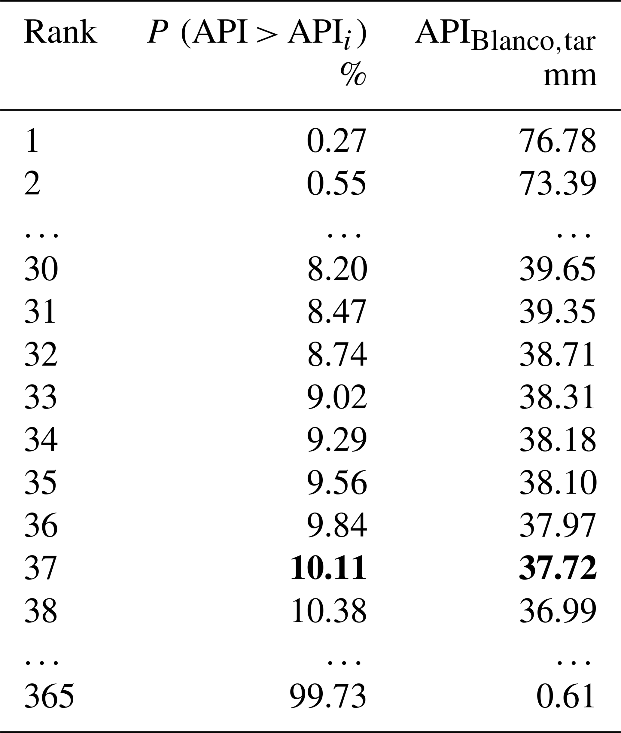
Table A2The (bold) API value found in Table A1 is compared to the sample of API values estimated for the donor years (i.e., 1948–1963) at the donor basin (i.e. Blanco River, TX). The closest values are considered and the corresponding percentiles estimated (in bold).
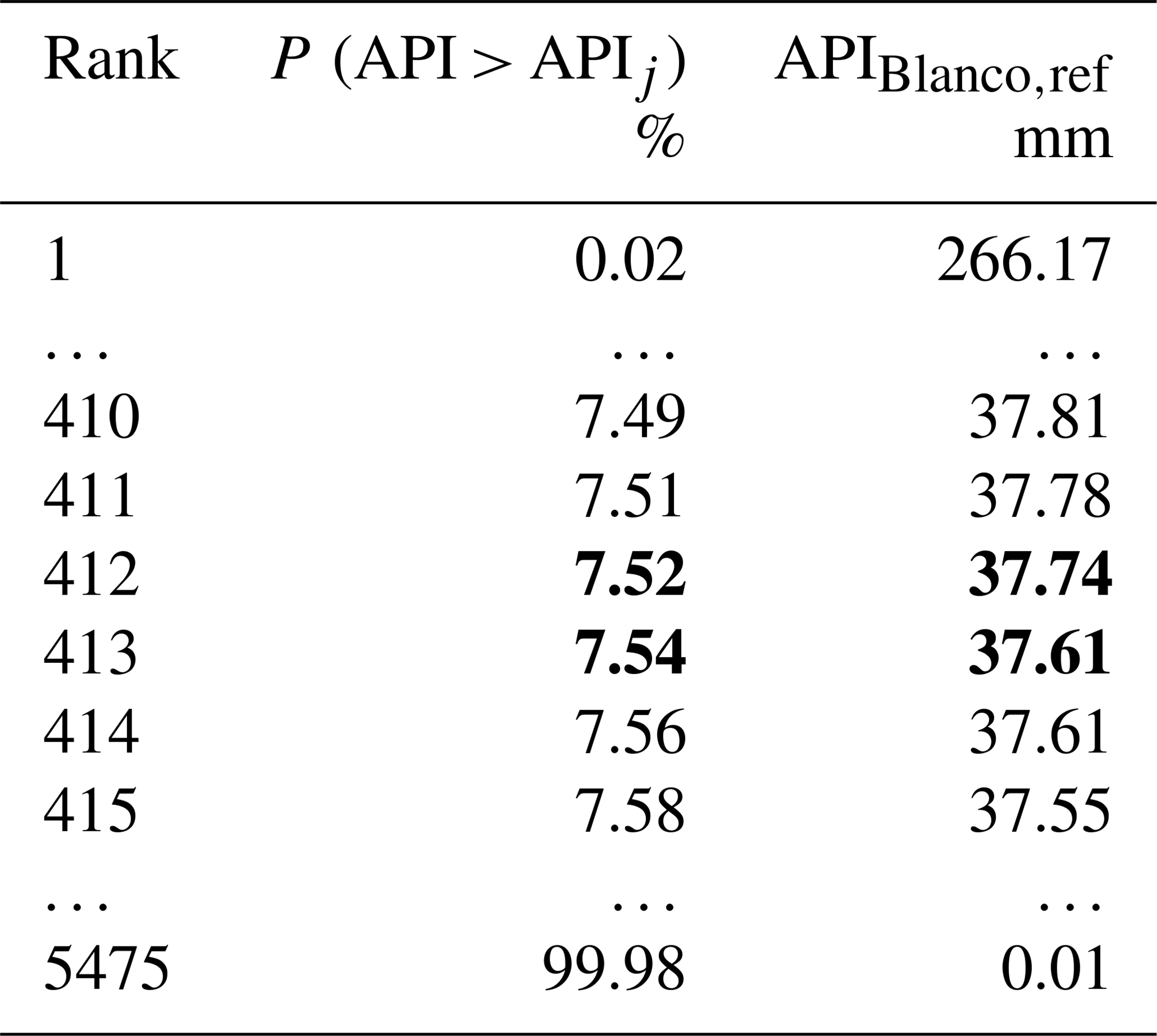
Table A3The (bold) percentiles identified in Table A2 are used here to retrieve the corresponding streamflow values gauged during the donor years (i.e., 1948–1963) at the target basin (i.e., Bogue River, LA). Percentiles and the corresponding streamflow values are in bold.
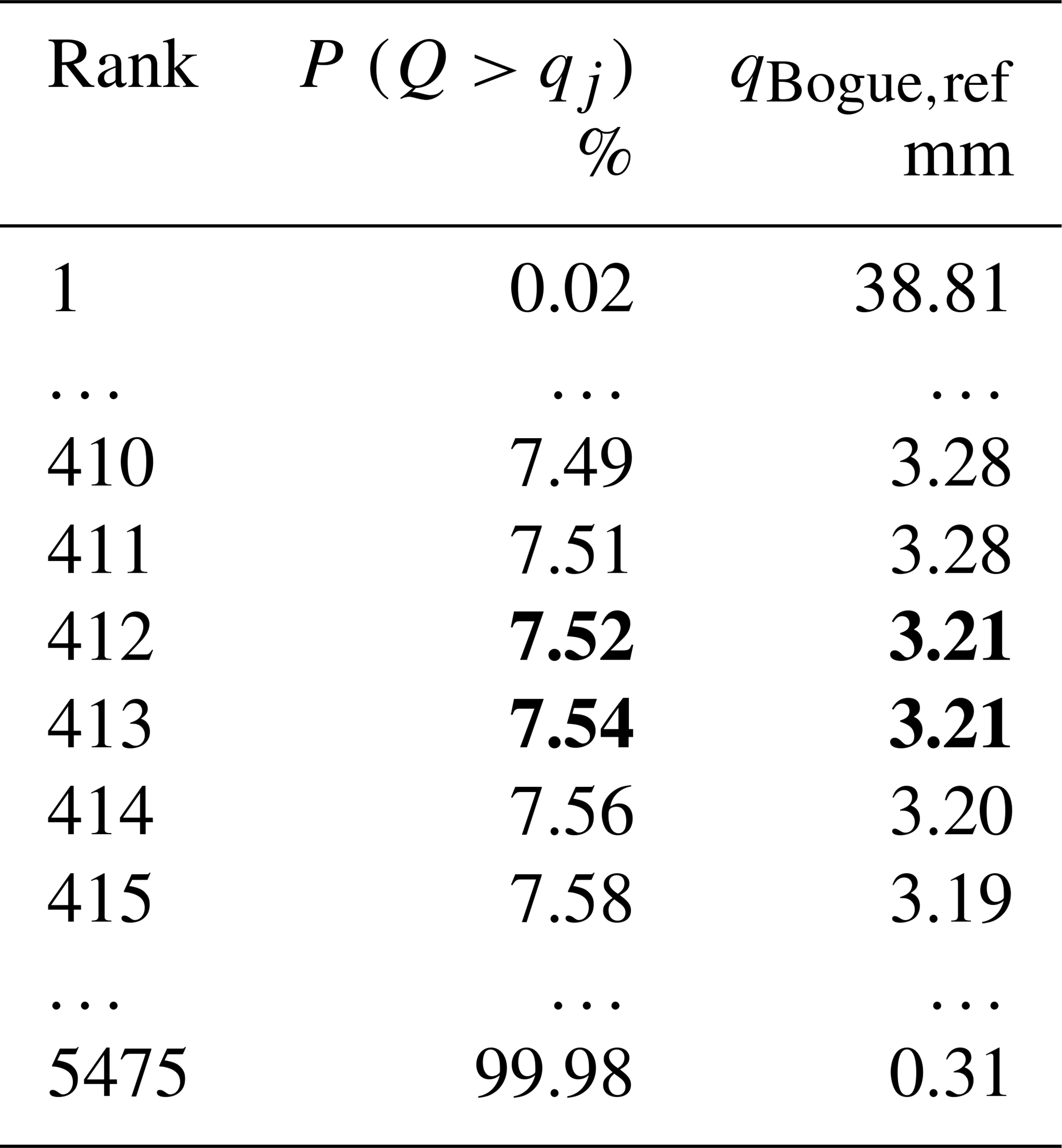
Table A4The initially unknown streamflow value corresponding to the 10.11th percentile estimated for the target year (i.e., 1968–1969) at the target basin (i.e., Bogue River, LA).
The streamflow is obtained from USGS National Water Information System (NWIS), available at http://water.usgs.gov/nwis (last access: 15 April 2020) (USGS, 2020). Mean areal precipitation and climatic potential evaporation were supplied by the National Centers for Environmental Information, formerly the National Climate Data Center (NCDC), at daily resolution (https://www.ncdc.noaa.gov/data-access, last access: 15 April 2020) (NOAA, 2020).
AB and ER jointly developed the concept and the methodology of the study. HK and ER performed the computations and the analysis for the case study. ER wrote the first draft of the manuscript. The manuscript was revised by ER and AB.
The authors declare that they have no conflict of interest.
The authors would like to express their gratitude to William Farmer, Thomas Over and Francesco Serinaldi for the fruitful discussion that consistently improved the paper.
Elena Ridolfi has been supported by the Centre of Natural Hazards and Disaster Science (CNDS) in Sweden (https://www.cnds.se/, last access: 15 April 2020).
This paper was edited by Stacey Archfield and reviewed by William Farmer and Thomas Over.
Alaouze, C.: Transferable water entitlements which satisfy heterogeneous risk preferences, Aust. J. Agricult. Econ., 35, 197–208, 1991.
Archfield, S. A. and Vogel, R. M.: Map correlation method: Selection of a reference streamgage to estimate daily streamflow at ungaged catchments, Water Resour. Res., 46, W10513, https://doi.org/10.1029/2009WR008481, 2010.
Bárdossy, A., Huang, Y., and Wagener, T.: Simultaneous calibration of hydrological models in geographical space, Hydrol. Earth Syst. Sci., 20, 2913–2928, https://doi.org/10.5194/hess-20-2913-2016, 2016.
Blöschl, G., Sivapalan, M., Thorsten, W., Viglione, A., and Savenije, H.: Runoff prediction in ungauged basins: Synthesis across Processes, Places and Scales, Cambridge University Press, Cambridge, 2013.
Bonta, J. V. and Cleland, B.: Incorporating natural variability, uncertainty, and risk into water quality evaluations using duration curves, J. Am. Water Resour. Assoc., 39, 1481–1496, https://doi.org/10.1111/j.1752-1688.2003.tb04433.x, 2003.
Brown, A. E., Zhang, L., McMahon, T. A., Western, A. W., and Vertessy, R. A.: A review of paired catchment studies for determining changes in water yield resulting from alterations in vegetation, J. Hydrol., 310, 28–61, https://doi.org/10.1016/j.jhydrol.2004.12.010, 2005.
Budyko, M. I.: Climate and Life, Academic Press, San Diego, California, USA, 1974.
Carrillo, G., Troch, P. A., Sivapalan, M., Wagener, T., Harman, C., and Sawicz, K.: Catchment classification: Hydrological analysis of catchment behavior through process-based modeling along a climate gradient, Hydrol. Earth Syst. Sci., 15, 3411–3430, https://doi.org/10.5194/hess-15-3411-2011, 2011.
Castellarin, A., Burn, D., and Brath, A.: Assessing the effectiveness of hydrological similarity measures for flood frequency analysis, J. Hydrol., 241, 270–285, 2001.
Castellarin, A., Camorani, G., and Brath, A.: A stochastic model of flow duration curves, Adv. Water Resour., 30, 937–953, https://doi.org/10.1029/93WR01409, 2007.
Castellarin, A., Botter, G., Hughes, D., Liu, S., Ouarda, T., Parajka, J., Post, M., Sivapalan, M., Spence, C., Viglione, A., and Vogel, R.: Prediction of flow duration curves in ungauged basins, in: Runoff prediction in ungauged basins: Synthesis across Processes, Places and Scales, edited by: Blöschl, G., Sivapalan, M., Wagener, T., Viglione, A., and Savenije, H., Cambridge University Press, Cambridge, 2013.
Chow, V. T.: Handbook of applied hydrology, Mc-Graw Hill Book Co., New York, NY, 1964.
Dingman, S. L.: Planning level estimates of the value of reservoirs for water supply and flow augmentation in New Hampshire, J. Am. Water Resour. Assoc., 17, 684–690, https://doi.org/10.1111/j.1752-1688.1981.tb01277.x, 1981.
Duan, Q., Schaake, J., Andreassian, V., Franks, S., Goteti, G., Gupta, H., Gusev, Y., Habets, F., Hall, A., Hay, L., Hogue, T., Huang, M., Leavesley, G., Liang, X., Nasonova, O., Noilhan, J., Oudin, L., Sorooshian, S., Wagener, T., and Wood, E.: Model Parameter Estimation Experiment (MOPEX): An overview of science strategy and major results from the second and third workshops, J. Hydrol., 320, 3–17, 2006.
Farmer, W. H., Archfield, S. A., Over, T. M., Hay, L. E., LaFontaine, J. H., and Kiang, J. E.: A comparison of methods to predict historical daily streamflow time series in the southeastern United States, US Geological Survey Scientific Investigations Report 2014-5231, p. 34, https://doi.org/10.3133/sir2014-5231, 2014.
Fennessey, N. and Vogel, R. M.: Regional Flow-Duration Curves for Ungauged Sites in Massachusetts, J. Water Resour. Plan. Manage., 116, 530–549, https://doi.org/10.1061/(ASCE)0733-9496(1990)116:4(530), 1990.
Franchini, M. and Suppo, M.: Regional analysis of flow duration curves for a limestone region, Water Resour. Manage., 10, 199–218, 1996.
Ganora, D., Claps, P., Laio, F., and Viglione, A.: An approach to estimate nonparametric flow duration curves in ungauged basins, Water Resour. Res., 45, 1–10, https://doi.org/10.1029/2008WR007472, 2009.
Hänggi, P. and Weingartner, R.: Variations in Discharge Volumes for Hydropower Generation in Switzerland, Water Resour. Manage., 26, 1231–1252, https://doi.org/10.1007/s11269-011-9956-1, 2012.
Hughes, D. A. and Smakhtin, V. Y.: Daily flow time series patching or extension: a spatial interpolation approach based on flow duration curves, Hydrolog. Sci. J., 41 851–871, https://doi.org/10.1080/02626669609491555, 1996.
Jarvis, A., Reuter, H. I., Nelson, A., and Guevara, E.: Hole-filled seamless SRTM data V4, International Centre for Tropical Agriculture (CIAT), available at: http://srtm.csi.cgiar.org (last access: 15 April 2020), 2008.
Jothityangkoonad, C. and Sivapalan, M.: Framework for exploration of climatic and landscape controls on catchment water balance, with emphasis on inter-annual variability, J. Hydrol., 371, 154–168, 2009.
Kohler, M. and Linsley, R.: Predicting the runoff from storm rainfall, US Weather Bureau Research Paper No. 34, US Weather Bureau, Washington, p. 10, 1951.
Linsley, R., Kohler, M., and Paulhus, J.: Applied Hydrology, 1st Edn., McGraw-Hill, New York, 1949.
Massey, F. J.: The Kolmogorov-Smirnov Test for Goodness of Fit, J. Am. Stat. Assoc., 46, 68–78, 1951.
McMahon, T. A., Laaha, G., Parajka, J., Peel, M., Savenije, H., Sivapalan, M., Szolgay, J., Thompson, S. E., Viglione, A., Wood, E. A., and Yang, D.: Prediction of annual runoff in ungauged basins, in: Runoff Prediction In Ungauged Basins: Synthesis Across Across Processes, Places and Scales, edited by: Bloschl, G., Sivapalan, M., Wagener, T., Viglione, A., and Savenjie, H., Cambridge University Press, Cambridge, 2013.
Mohamoud, Y. M.: Prediction of daily flow duration curves and streamflow for ungauged catchments using regional flow duration curves, Hydrolog. Sci. J., 53, 706–724, https://doi.org/10.1623/hysj.53.4.706, 2008.
Montanari, L., Sivapalan, M., and Montanari, A.: Investigation of dominant hydrological processes in a tropical catchment in a monsoonal climate via the downward approach, Hydrol. Earth Syst. Sci., 10, 769–782, https://doi.org/10.5194/hess-10-769-2006, 2006.
Nash, J. E. and Sutcliffe, J. V.: River flow forecasting through conceptual models part I – a discussion of principles, J. Hydrol., 10, 282–290, 1970.
NOAA: Data Access, available at: https://www.ncdc.noaa.gov/data-access, last access: 15 April 2020.
Pugliese, A., Castellarin, A., and Brath, A.: Geostatistical prediction of flow–duration curves in an index-flow framework, Hydrol. Earth Syst. Sci., 18, 3801–3816, https://doi.org/10.5194/hess-18-3801-2014, 2014.
Pugliese, A., Farmer, W. H., Castellarin, A., Archfield, S. A., and Vogel, R. M.: Regional flow duration curves: Geostatistical techniques versus multivariate regression, Adv. Water Resour., 96, 11–22, https://doi.org/10.1016/j.advwatres.2016.06.008, 2016.
Quimpo, R. G., Alejandrino, A. A., and McNally, T. A.: Regionalized flow duration for Philippines, J. Water Resour. Plan. Manage., 109, 320–330, 1983.
Rianna, M., Russo, F., and Napolitano, F.: Stochastic index model for intermittent regimes: from preliminary analysis to regionalisation, Nat. Hazards Earth Syst. Sci., 11, 1189–1203, https://doi.org/10.5194/nhess-11-1189-2011, 2011.
Rianna, M., Efstratiadis, A., Russo, F., Napolitano, F., and Koutsoyiannis, D.: A stochastic index method for calculating annual flow duration curves in intermittent rivers, Irrig. Drain., 62, 41–49, https://doi.org/10.1002/ird.1803, 2013.
Ridolfi, E., Rianna, M., Trani, G., Alfonso, L., Di Baldassarre, G., Napolitano, F., and Russo, F.: A new methodology to define homogeneous regions through an entropy based clustering method, Adv. Water Resour., 96, 237–250, 2016.
Scott, D., Prinsloo, F., Moses, G., Mehlomakulu, M., and Simmers, A.: A re-analysis of the South African catchment afforestation experimental data, Report 810/1/00, Tech. rep., Water Research Commission, Pretoria, 2000.
Smakhtin, V. Y.: Generation of natural daily flow time-series in regulated rivers using a non-linear spatial interpolation technique, Regul. Rivers Res. Manage., 15, 311–323, 1999.
Smakhtin, V. Y.: Low flow hydrology: A review, J. Hydrol., 240, 147–186, 2001.
Smakhtin, V. Y. and Masse, B.: Continuous daily hydrograph simulation using duration curves of a precipitation index, Hydrol. Process., 14, 1083–1100, https://doi.org/10.1002/(SICI)1099-1085(20000430)14:6<1083::AID-HYP998>3.0.CO;2-2, 2000.
Smakhtin, V. Y., Hughes, D. A., and Creuse-Naudin, E.: Regionalization of daily flow characteristics in part of the Eastern Cape, South Africa, Hydrolog. Sci. J., 42, 919–936, https://doi.org/10.1080/02626669709492088, 1997.
Sugimoto, T., Bárdossy, A., Pegram, G. G. S., and Cullmann, J.: Investigation of hydrological time series using copulas for detecting catchment characteristics and anthropogenic impacts, Hydrol. Earth Syst. Sci., 20, 2705–2720, https://doi.org/10.5194/hess-20-2705-2016, 2016.
USGS: USGS Water Data for the Nation, available at: http://water.usgs.gov/nwis, last access: 15 April 2020.
Vogel, R. M.: Flow Duration Curves. I: New interpretation and confidence intervals, J. Water Resour. Plan. Manage., 120, 485–504, https://doi.org/10.1017/CBO9781107415324.004, 1994.
Vogel, R. M., Sieber, J., Archfield, S. A., Smith, M. P., Apse, C. D., and Huber-Lee, A.: Relations among storage, yield, and instream flow, Water Resour. Res., 43, W05403, https://doi.org/10.1029/2006WR005226, 2007.
Weibull, W.: A statistical theory of the strength of materials, Ing. Vetensk. Akad. Handl., 151, 1–45, 1939.
Weiss, M. S.: Modification of the Kolmogorov-Smirnov statistic for use with correlated data, J. Am. Stat. Assoc., 73, 872–875, https://doi.org/10.1080/01621459.1978.10480116, 1978.
Westerberg, I. K., Guerrero, J.-L., Younger, P. M., Beven, K. J., Seibert, J., Halldin, S., Freer, J. E., and Xu, C.-Y.: Calibration of hydrological models using flow-duration curves, Hydrol. Earth Syst. Sci., 15, 2205–2227, https://doi.org/10.5194/hess-15-2205-2011, 2011.
Worland, S. C., Steinschneider, S., Farmer, W., Asquith, W., and Knight, R.: Copula Theory as a Generalized Framework for Flow-Duration Curve Based Streamflow Estimates in Ungaged and Partially Gaged Catchments, Water Resour. Res., 55, 9378–9397, 2019.
Xu, X.: Methods in Hypothesis Testing, Markov Chain Monte Carlo and Neuroimaging Data Analysis, PhD Thesis, Harvard, available at: https://dash.harvard.edu/handle/1/11108711 (last access: 15 April 2020), 2014.
Yu, P.-S. and Yang, T.-C.: Using synthetic flow duration curves for rainfall-runoff model calibration at ungauged sites, Hydrol. Process., 14, 117–133, https://doi.org/10.1002/(SICI)1099-1085(200001)14:1<117::AID-HYP914>3.0.CO;2-Q, 2000.