the Creative Commons Attribution 4.0 License.
the Creative Commons Attribution 4.0 License.
 | 23 Apr 2020
A new uncertainty estimation approach with multiple datasets and implementation for various precipitation products
Jan Polcher
Ching-Sheng Huang
Ensemble estimates based on multiple datasets are frequently applied once many datasets are available for the same climatic variable. An uncertainty estimate based on the difference between the ensemble datasets is always provided along with the ensemble mean estimate to show to what extent the ensemble members are consistent with each other. However, one fundamental flaw of classic uncertainty estimates is that only the uncertainty in one dimension (either the temporal variability or the spatial heterogeneity) can be considered, whereas the variation along the other dimension is dismissed due to limitations in algorithms for classic uncertainty estimates, resulting in an incomplete assessment of the uncertainties. This study introduces a three-dimensional variance partitioning approach and proposes a new uncertainty estimation (Ue) that includes the data uncertainties in both spatiotemporal scales. The new approach avoids pre-averaging in either of the spatiotemporal dimensions and, as a result, the Ue estimate is around 20 % higher than the classic uncertainty metrics. The deviation of Ue from the classic metrics is apparent for regions with strong spatial heterogeneity and where the variations significantly differ in temporal and spatial scales. This shows that classic metrics underestimate the uncertainty through averaging, which means a loss of information in the variations across spatiotemporal scales. Decomposing the formula for Ue shows that Ue has integrated four different variations across the ensemble dataset members, while only two of the components are represented in the classic uncertainty estimates. This analysis of the decomposition explains the correlation as well as the differences between the newly proposed Ue and the two classic uncertainty metrics. The new approach is implemented and analysed with multiple precipitation products of different types (e.g. gauge-based products, merged products and GCMs) which contain different sources of uncertainties with different magnitudes. Ue of the gauge-based precipitation products is the smallest, while Ue of the other products is generally larger because other uncertainty sources are included and the constraints of the observations are not as strong as in gauge-based products. This new three-dimensional approach is flexible in its structure and particularly suitable for a comprehensive assessment of multiple datasets over large regions within any given period.


With the technical developments in monitoring natural climate variables and the increasing knowledge of the physical mechanisms in the climate system, many institutes have the ability to provide different kinds of climate datasets. Taking precipitation, which is the dominant variable in the land water cycle, as an example, there are point measurements, such as GHCN-D (global historical climatology network-daily, Menne et al., 2012), gridded products based on gauge measurements and interpolation (e.g. CRU, Harris et al., 2014), products derived from remote sensing (e.g. the Tropical Rainfall Measuring Mission – TRMM), reanalysis datasets (e.g. NCEP) and estimates from models (e.g. GCMs). These products have been developed using different original data, technologies and model settings for various purposes (Phillips and Gleckler, 2006; Tapiador et al., 2012; Beck et al., 2017; Sun et al., 2018). As a result, there are differences between the various products due to measurement errors, model biases, or chaotic noise. The uncertainty is thus regarded as the deviation of these model results from their real values.
However, the real values are difficult to measure and the uncertainties are difficult to remove from the datasets. Thus, using ensembles consisting of multiple datasets to generate a weighted average has become very popular in climate-related research. The ensemble means of multiple datasets are considered more reliable estimates than a single dataset. For example, IPCC uses 42 CMIP5 (Coupled Model Intercomparison Project Phase 5) models to show historical temperature changes and 39 CMIP5 models to average future temperature projections in a RCP 8.5 scenario (Fig. SPM.7 in IPCC, 2013b). Schewe et al. (2014) use nine global hydrological models to evaluate global water scarcity under climate change. GLDAS (Global Land Data Assimilation System) involves four different land surface models (Rodell et al., 2004) and GRACE (Gravity Recovery and Climate Experiment) provides estimates from three independent institutes (Landerer and Swenson, 2012). Using multiple datasets reduces the dependence on a single dataset and eliminates the random variations associated with biases or noise in each single model estimate.
Along with the ensemble means, uncertainty information is recommended to be presented because the level of uncertainty determines the reliability of the ensemble results. In general, uncertainties can be quantified as the range of maximum and minimum values (i.e. Vmax−Vmin), the value difference at different quantiles (e.g. V5 %−V95 %), the consistency of models (ratio of models following a certain pattern to the total number of models), the variation (σ2) or the standard deviation (σ) of multiple model estimations. These metrics describe the differences between multiple model estimates in different aspects. Among the metrics, the standard deviation (σ) is the most used because it has the same unit as the original dataset. Moreover, it is less sensitive to extreme samples and to the number of datasets used for the investigation. The ratio of the standard deviation (σ) to the mean value (μ), the so-called coefficient of variance (CV), representing the dispersion or spread of the distribution of various ensemble members (Everitt, 2013), is a unitless value which also shows the degree of uncertainty efficiently.
Depending on the purpose of data evaluation, the uncertainty between the datasets can be displayed or visualized in space to show the spatial heterogeneity. For example, the predicted future temperature increase has a higher significance in different models in the northern high latitudes than in the middle latitudes (Box TS.6 Fig. 1 in IPCC, 2013a). Another typical implementation is to evaluate the evolution of the uncertainty over time. In general, the range of the uncertainty decreases in the historical period over time because more observations have been accessible recently. But the uncertainty increases in future projections because of the increasing spread of model estimates (Fig. SPM.7 in IPCC, 2013b), indicating a decreasing consistency but increasing variation across various datasets.
The two kinds of ways can easily show the spatial distribution or the temporal evolution of the uncertainty. But a shortcoming is apparent, as the variation along one dimension (time or space) has to be collapsed to generate the mean values when we attempt to assess the uncertainty for the other dimension (space or time). For example, the averaging over a specific region to obtain the spatial mean is estimated at each time step before obtaining the temporal evolution of the model uncertainty (red flowcharts in Fig. 1). In contrast, averaging over a certain temporal period to obtain the temporal mean is necessary for each grid cell when estimating the spatial variations of model uncertainties (blue flowcharts in Fig. 1). The averaging, in either dimension, means a loss of information about the variation in the data. Any changes in the variation that leave the mean values unchanged will not be propagated to the global uncertainty estimation. The result of this is that the variations between datasets are not fully considered when estimating the uncertainties. In other words, neither of the uncertainty estimates can represent the whole of the differences between multiple datasets. The uncertainty can be underestimated, and the similarity of the datasets thus overestimated. Indeed, the current literature has not paid attention to the neglect of variation after averaging as well as its influence on the assessment of the uncertainty.
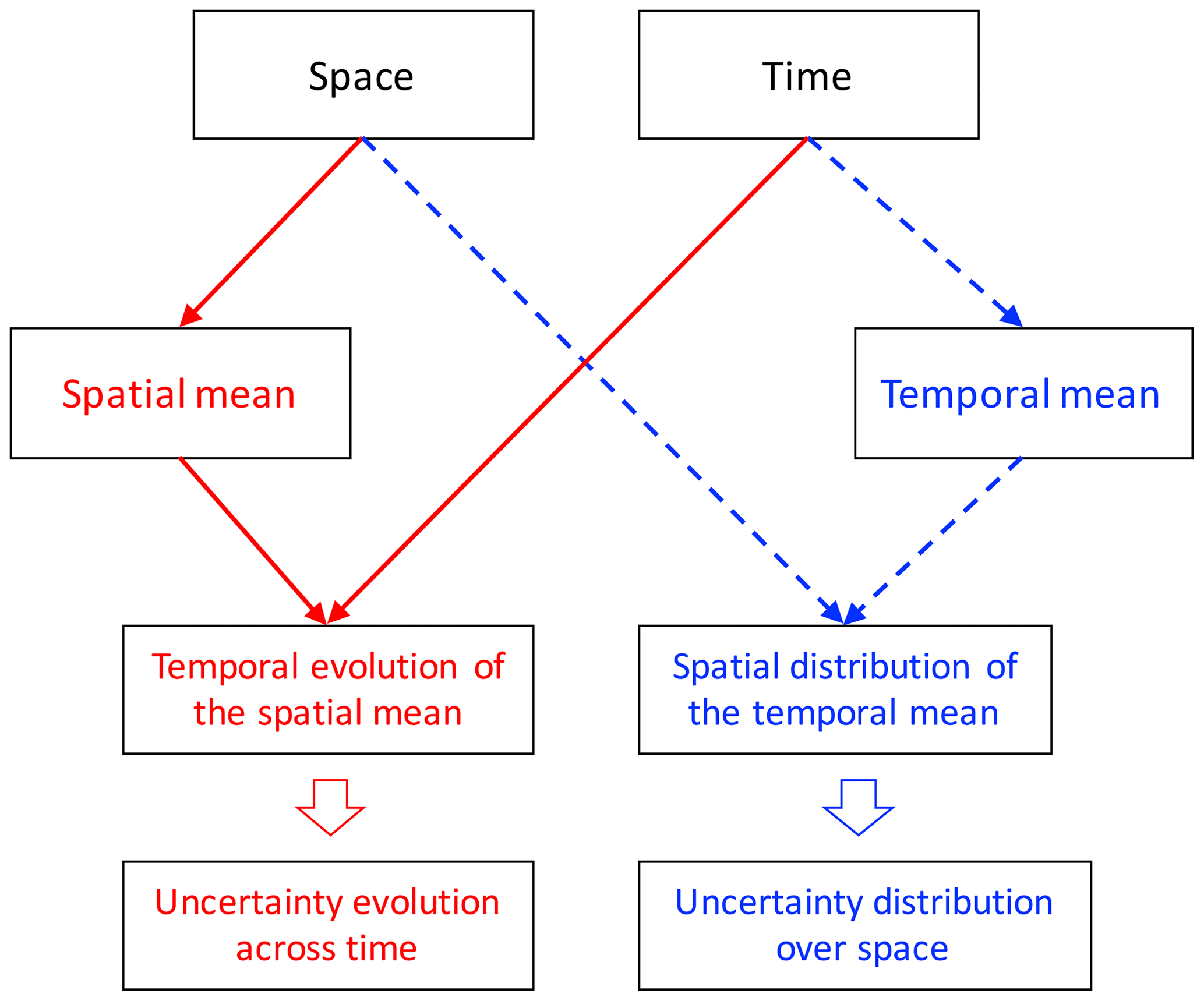
Figure 1Two classic uncertainty assessments in the current literature: the temporal evolution of the model uncertainty (flowcharts in red) and the spatial distribution of the model uncertainty (flowcharts in blue). Each of these uncertainty estimates was averaged over one of the dimensions, either space or time, which will lead to loss of information about the corresponding dimension.
The total variation across multiple datasets is contributed by the spatial heterogeneity, temporal variability and the model uncertainties. To some degree, the model uncertainty is similar to other dimensions as a variation along a third dimension (ensemble dimension). The key to evaluating the model uncertainty is to decompose the variation caused by differences between the datasets from the other two contributors. Although decomposing the variation by means of ANalysis Of VAriance (ANOVA) is often seen in hydro-meteorological studies, this is designed to separate the process uncertainties generated in different model processes that propagate to the final variation. For example, Déqué et al. (2007) decomposed the uncertainties of regional climate models (RCMs) into four sources of uncertainty: sampling uncertainty, model uncertainty, radiative uncertainty and boundary uncertainty. Bosshard et al. (2013) decomposed the uncertainty in river streamflow projections to uncertainties from climate models, statistical post-processing schemes and hydrological models. These implementations differ from the purpose of the present study because they fail to separate the uncertainties from the spatiotemporal variations because spatiotemporal averaging was already applied in the estimation process. Sun et al. (2010, 2012) for the first time decomposed the total variation into temporal variation and spatial heterogeneity. They concluded that the variations along the spatial dimension contributed more to the total variation than did the temporal variabilities. However, their approach is only valid for one single dataset and is thus not able to evaluate the uncertainties if multiple datasets describe the same variable. But a generalized approach should be based on Sun's work, as one more dimension can be added for a specific analysis of the uncertainties.
In the present study, we aim to introduce a new approach to estimating uncertainty of multiple datasets. The new uncertainty metric should avoid any averaging over time or space, so that all information along each of these two dimensions can be maintained for the assessment of the uncertainty. Multiple precipitation products will be used to display the results and explain the specifics of the new approach. In Sect. 2, the details of the three-dimensional variance partitioning approach are introduced. The characteristics of multiple precipitation datasets and estimations of two other classic uncertainty metrics are shown in Sect. 3. The results of the new approach for precipitation products are discussed in terms of the types of precipitation datasets in Sect. 4. The differences between the new uncertainty estimate and two selected classic metrics used in uncertainty analysis are analysed and discussed in Sect. 5. A discussion and some conclusions follow in Sect. 6.
2.1 Mathematical derivation
Multiple datasets recording the same climatic variable should be reorganized into a three-dimensional database, using the dimensions of (1) time with a regular time interval (e.g. monthly or annual), (2) space with regular spatial units, with all the grids re-organized into one dimension from the original longitude–latitude grids, and (3) ensemble as the third dimension describing the different ensemble datasets. Thus, the dataset array can be re-organized to be
with the ith time step (), jth grid (), and kth ensemble member or ensemble model ().
We define the three dimensions to be time, space and ensemble dimension, and the means for these three dimensions to be the temporal mean, spatial mean and ensemble mean. The corresponding variances are referred to as the temporal variance, spatial variance, and ensemble variance. We also define the grand mean (μ), grand variance (σ2) and total sum of squares (SST) (or total variation) across the entire database:
The total variation receives contributions from the variations along all three dimensions (Eq. 4). It can be reformulated as an expression in terms of the variations along each of the three different dimensions. For instance, the derivation of the total variation can start from the third ensemble dimension. For a specific kth ensemble member, the grand mean is formulated as , leading to the total sum of squares being rewritten as
The SST can be further expanded and rearranged as
where σ2(μts) is the variation of the grand mean for each ensemble member and is the grand variance in the spatial and temporal dimensions for the ensemble member k. Moreover, can be split using the mean of the spatial variation at each time step and the variation of the spatial mean , denoted as in Eq. (9) with its derivation given in Eqs. (10)–(17).
For a specific dataset k, the grand mean μts[k] at the spatiotemporal scale is
The total sum of squares of the differences from the grand mean of this ensemble member is
and the grand variance is
The derivation can start from either the spatial dimension or the temporal dimension. If the derivation starts from the spatial dimension, Eq. (11) can be rewritten by incorporating the spatial mean of each time step :
This can be expanded and then rearranged as
The grand variance of this specific dataset is Eq. (17) (identical to Eq. 9).
Here, is the mean of the spatial variation at each time step and is the variation of the spatial mean, or if we started the derivation from the time dimension, the grand variance can be split using the average of the temporal variation from all regions and the spatial variation of the temporal mean :
With Eqs. (9) or (17) and (18), we obtain
Substituting Eq. (19) into (8) results in
The first term on the right-hand side of Eq. (20) can be transformed to
where is the mean value across ensemble members of the spatial variation of the temporal mean, and represents the grand mean of , which is the grand variance across the temporal and ensemble dimensions. Eq. (20) then becomes
where denotes the mean value across ensemble members of the temporal variation of the spatial mean, denotes the grand mean of , the grand variance across space and ensemble dimensions, and denotes the variation across ensemble members of the spatial–temporal means μts.
Similarly, the global derivation of SST can start from any of the other two dimensions (i.e. space or time). This derivation can then be formulated as
where each variable is defined in Appendix A. Averaging these three expressions of SST defined in Eqs. (22)–(24) leads to
With the total number of degrees of freedom being , the grand variance is expressed as
where Vt, Vs and Ve denote the temporal, spatial and ensemble variances, respectively. An illustration of the present approach is shown in Fig. 2 to facilitate the understanding of the partitioning results. The original database, consisting of multiple datasets, is re-organized into three dimensions (grey in the centre). Zones with different colours represent different processes of the original database from different dimensions (see the details in the caption of Fig. 2 and Appendix A).
Note that the ensemble variance Ve in Eq. (26) is a combination of several variations across the ensemble members. The four components are the variations of temporal and spatial values (, zone B3), temporal mean (, zone C5), spatial mean (, zone C6) and the grand variance of the spatiotemporal mean for a single ensemble member (, zone F3). Similarly, the other variances only rely on the variances in the corresponding dimension, which shows the independence of the three dimensions. This also is an illustration of the fact that the uncertainty across ensemble members is similar to the temporal variation and spatial heterogeneity.
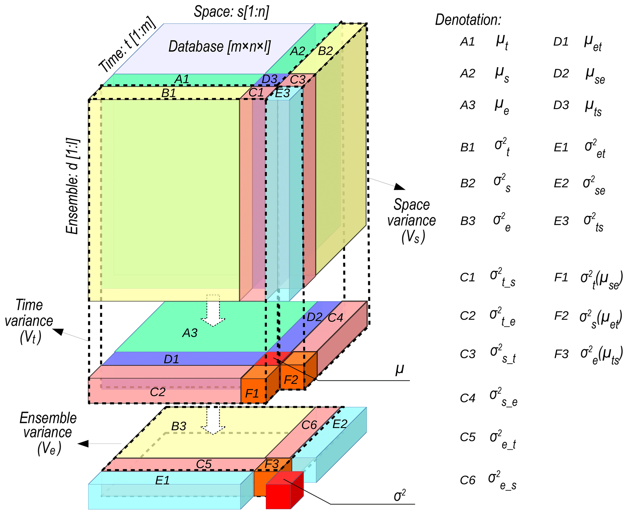
Figure 2Partitioning the temporal–spatial-ensemble variance. The original database is re-organized into three dimensions: time, space and ensemble. Zones with different colours represent different processes based on the original database through different dimensions. The labels of the zones are listed on the right; detailed definitions can be found in Appendix A. The grand variance is σ2 and the grand mean is μ. The subscripts t, s, and e indicate dimensions of time, space and ensemble, respectively. In Zone A, μx shows the mean values across the x dimension (x= t, s or e); in Zone B, indicates the variation across the x dimension; in Zone C, indicates the variation across the x dimension of μy (y= t, s or e); in Zone D, μxy indicates the means across the x and y dimensions; in Zone E, indicates the variation across the x and y dimensions; in Zone F, indicates the variation across the x dimension of the means across the y and z dimensions (z= t, s or e).
2.2 Definitions of the metrics for model uncertainty
Although the total variation is a result of contributions from the spatial heterogeneity, temporal variability and the uncertainties across different datasets, we mainly focus on the variance in the ensemble dimension because the spatial or temporal variation is natural for climatic variables. The uncertainty of ensemble members is normalized as the ratio of the square root of the ensemble variance (Ve) to the grand mean value of the datasets (μ).
Two classic metrics used for uncertainty estimates are also introduced for comparison. For each basic spatial unit (in the present study this means a grid cell), we can estimate the temporal mean of the target variable in each ensemble dataset as μt[j,k], represents the spatial unit and represents the index of the dataset. Then we can estimate the variations across different ensemble datasets of the mean values as (expressed as in this study). The spatial distribution of the shows the magnitude of the model uncertainty over space and its root σe_t[j] is the model deviation at each spatial unit. The estimate of this model deviation over the entire region can be expressed as
For each spatial unit, () can take a different value. The values for all the grid cells are averaged to obtain , which shows the general magnitude of the ensemble variation over space. The quantity N.s.std is normalized as the ratio of the square root of the averaged variations to the grand mean of all the datasets μ.
Similarly, the model uncertainty can be normalized as the ratio of the square root of the averaged ensemble variation but at different time steps to the entire means:
where () is the variation across different datasets of the spatial means of each product at each time unit .
The two uncertainty estimates (Eqs. 28 and 29) correspond to the two classic metrics presented in the Introduction. We will compare Ue estimated by the newly proposed approach with these two classic metrics (N.t.std and N.s.std) to show their relations and differences.
2.3 Study area and data description
Mainland China has been selected as the study area because of its large area and different types of climate (Kottek et al., 2006). Ten different subregions have been defined to facilitate the comparisons and analysis of the strong spatial variations. The subregions are (1) Songhua River Basin, (2) Liao River Basin, (3) Hai River Basin, (4) Yellow River Basin, (5) Huai River Basin, (6) Yangtze River Basin, (7) Southeast China, (8) South China, (9) Southwest China, and (10) Northwest China; see Fig. 3. The entire Chinese mainland is numbered as the 11th region. Most of the subregions are natural river basins: this definition is more appropriate for water resource analysis than definitions using longitude–latitude grids or those based on administrative regions.
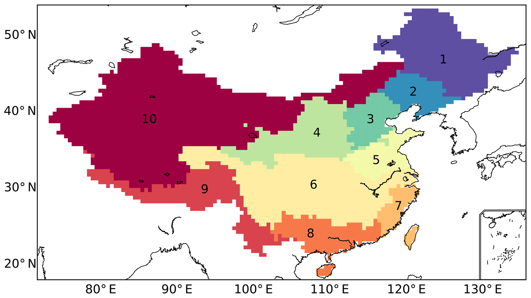
Figure 3Ten subregions are defined in this study. These subregions are mainly river basins (Regions 1–8), but 9 is Southwest China and 10 is Northwest China. Region 11 is the entirety of the Chinese mainland.
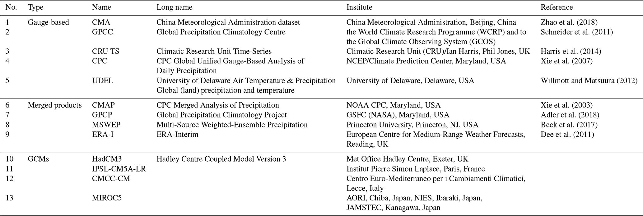
Precipitation is one of the climatic variables sensitive to large-scale atmospheric cycles and the local topography. Thirteen different precipitation datasets from various sources have been collected for comparison (Table 1). These datasets have been categorized into three groups according to the methods they used for generating the products, namely, gauge-based products, merged products and general circulation models (GCMs). The gauge-based products (namely, CMA, GPCC, CRU, CPC and UDEL) use data observed from global precipitation gauges. The density of the ground observation gauges, the representativeness of the gauges, and the interpolation algorithms for converting the gauge observations to a gridded dataset differ from product to product. The CMA (China Meteorological Administration) dataset has the densest distribution of gauges and probably has the best quality to capture the spatiotemporal variations of the precipitation over the study area. The CMA dataset is excluded when estimating the uncertainty of the gauge-based products: it is chosen as the reference dataset for comparison.
As for the merged precipitation products, the CMAP, GPCP and MSWEP use different sources of precipitation data (namely, gauge observations, satellite remote sensing, and atmospheric model re-analysis). These different precipitation sources are averaged using different weights. Thus, the differences between the three merged products are associated with the precipitation sources and the weight of the gauge observations. ERA-Interim is a re-analysis product: it uses near-real-time assimilation with data from global observations (Dee et al., 2011). Thus, the forecasting model is constrained by the observations and forced to follow the real system to some degree. Because of its use of observations, ERA-Interim also belongs to the category of merged products.
GCM precipitation is a pure model estimation because observations are not used to constrain the simulations. The implemented physical and numerical processes will affect the accuracy of the model results. The lack of constraints on the GCMs will cause them to not follow the actual synoptic variability and explore other trajectories in the solution space. Kay et al. (2015) repeatedly ran the same GCM with a very small shift in the initial conditions. But the small difference leads to an increasing spread in the model outputs after a number of running time steps (see Fig. 2 in Kay et al., 2015). Therefore, the uncertainty in GCMs can be attributed to the differences in the model structures, parameter settings, and the initial conditions as well. There are more than 20 kinds of different GCMs; only 4 of them have been chosen, randomly, to maintain the same number of datasets using the gauge-based products as those using merged products.
All the products of the three precipitation types, including CMA, are in gridded format. Although they differ in their original spatial resolution, all the products have been interpolated to a 0.5∘ spatial resolution to unify the spatial units. Annual average values are summed based on their original time steps (daily or monthly) and the overlap time span of all the datasets is from 1979 to 2005 for all the products.
Zhao et al. (2018)Schneider et al. (2011)Harris et al. (2014)Xie et al. (2007)Willmott and Matsuura (2012)Xie et al. (2003)Adler et al. (2018)Beck et al. (2017)Dee et al. (2011)Table 1Precipitation datasets used in this study. Three different precipitation groups have been identified according to the way the precipitation dataset is generated.
3.1 Spatial patterns of annual precipitation
The long-term annual mean precipitation (1979–2005) obtained by averaging the precipitation from multiple datasets in the corresponding precipitation group is mapped in Fig. 4. The annual mean precipitation obtained from the CMA dataset is 589.8 mm yr−1 (1.6 mm d−1) over the entire Chinese mainland. The gauge-based precipitation has the least bias (−4.1 mm yr−1, −0.7 % in percentage) compared to the CMA precipitation. The precipitation in the merged products and GCMs is larger than that of the CMA by 63.1 and 232.0 mm yr−1 (with the bias equal to +10.7 % and +39.3 %), respectively.
The spatial pattern of the annual precipitation shows a decreasing gradient from Southeast China (>1600 mm yr−1) to Northwest China (<400 mm yr−1) in CMA and all other three precipitation groups. However, they have different abilities to display the spatial gradient of the precipitation in some detail. For instance, abrupt precipitation changes rather than following the general gradient occur in some areas in CMA. This is probably caused by the sudden changes in topography (e.g. the northern Tienshan Mountains, the Qilian Mountains), which is not captured in the gauge-based products because some of the key gauges are not included in the production of the gauge-based products. The abrupt changes can be somehow represented by merged products and GCMs because the local variation due to topographic changes can be observed by other measurements or modelled by algorithms. The precipitation in the merged products and the GCMs is higher than that of CMA in the Himalayas, and particularly the GCMs show higher precipitation in the North Tibet Plateau as well as the southern part of the Hengduan Mountains. These differences show the general characteristics of the three types of precipitation products.
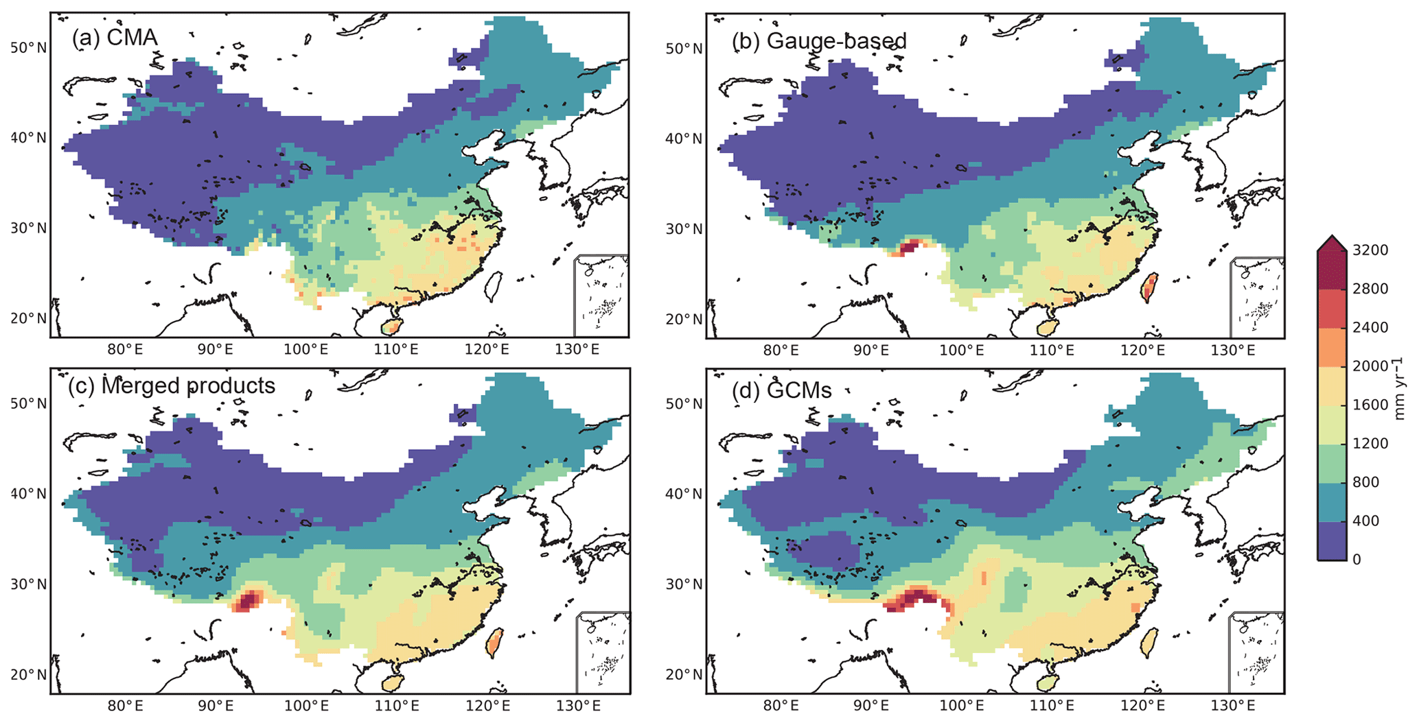
Figure 4Annual precipitation over a long-term period (1979–2005) for each group of precipitation datasets. (a) Annual precipitation of the CMA dataset, (b) ensemble means of the annual precipitation over the precipitation products in gauge-based precipitation excluding CMA, (c) ensemble mean of the annual precipitation of all merged products, and (d) ensemble means of the annual precipitation of all GCMs. The observations in Taiwan are not released in the CMA dataset.
3.2 Spatial distribution of model uncertainties
In addition to the precipitation differences in its long-term annual means, differences can be found between datasets within the same precipitation group. The spatial distribution of the model uncertainty for each precipitation group, which is expressed as the ensemble deviation of the annual precipitation from different precipitation products, is mapped in Fig. 5.
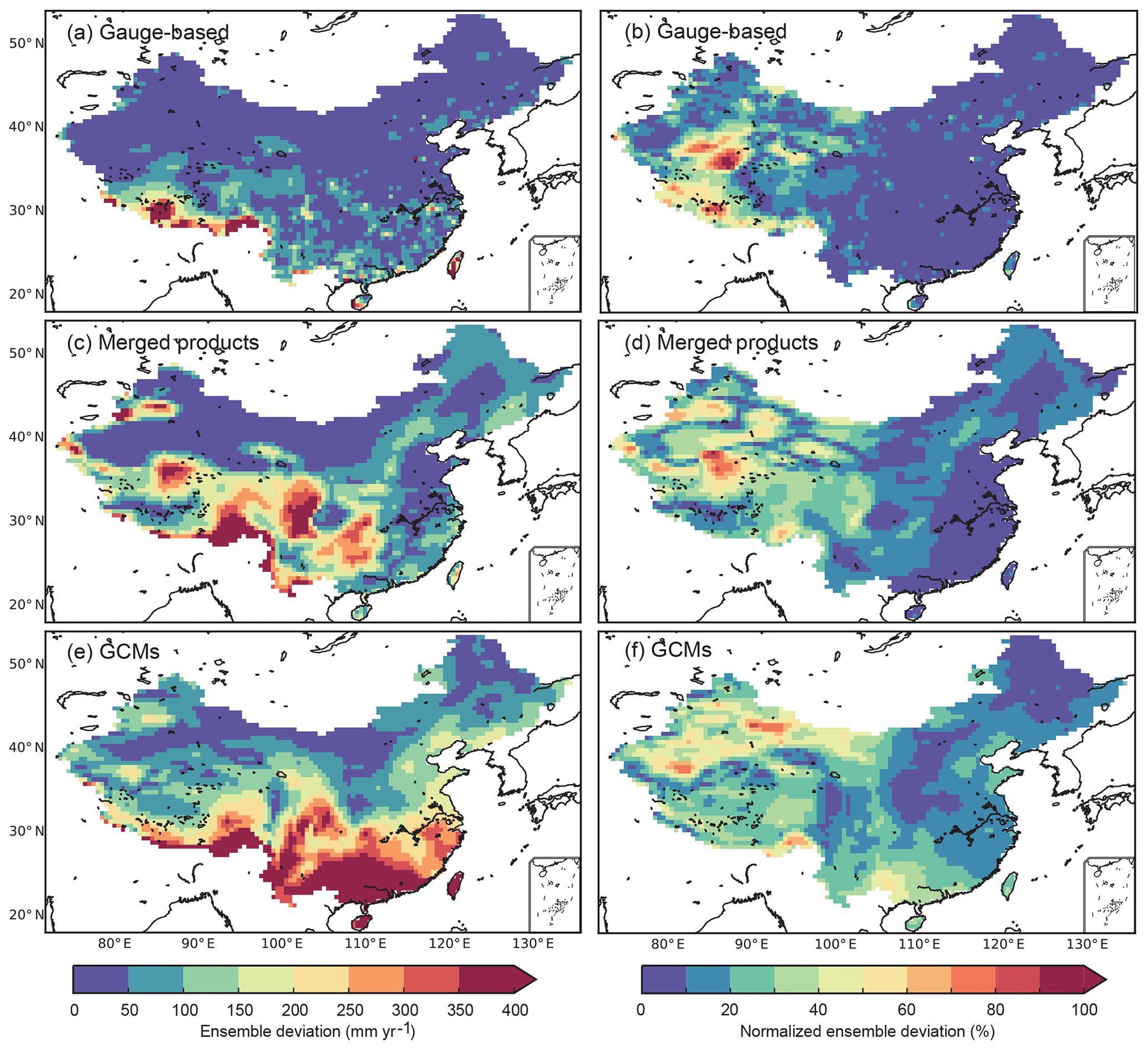
Figure 5Spatial distribution of model uncertainty in annual precipitation estimated by the ensemble products. The uncertainty is expressed as the standard deviation of the annual precipitation across ensemble precipitation products of a specific group (a, b: gauge-based products, middle: merged products, e, f: GCMs). (a, c, e) are the values of the uncertainty. (b, d, f) are the ratios of ensemble deviation to the ensemble means of the datasets in the corresponding group.
The ensemble deviation of the datasets based on gauge observations is small in most of the land area of China (<50 mm yr−1, Fig. 5a). Although the deviation is higher in the south of China (50–100 mm yr−1), the area is not continuous in space. The highest deviation occurs along the Himalayas, indicating a high variation across the observed datasets. Regarding the merged precipitation products, the deviation shows high values (>200 mm yr−1, Fig. 5c) in Southwest China (e.g. the Tibet Plateau, Yunnan Province, Guangxi Province). Moderate deviation is found in Northeast China, North China and Southeast China. The deviation of precipitation has a correlation with the topology, which indicates that the performances of the technologies used for the merged products are subject to the topologies as well. Compared to the gauge-based and merged products, the deviation of the selected GCMs has the highest value (>400 mm yr−1, Fig. 5e) in South China, indicating a significant model uncertainty of the annual precipitation between different GCMs.
The ratio of the ensemble deviation to the mean value, which shows the model uncertainty with no units, is very low in East China (<10 %, Fig. 5b). It is higher in West China, especially in the Himalayas and the North Tibet Plateau. Similarly to that of the gauge-based products, the uncertainty of the merged products has higher values in the west than in the east of China (Fig. 5d). The area with a deviation ratio less than 10 % is mainly distributed in Southeast China and is apparently smaller than that of the gauge-based products, showing a decreasing similarity among different merged products. The area with a moderate deviation ratio (10 %–40 %) increases compared to that of the gauge-based products, and the area is mostly in central and western China. The uncertainty estimated in the GCMs shows similar patterns in West China to that of the merged products, but with higher magnitudes in East China (Fig. 5f). Only the area in the northeast and part of central China features small uncertainty, less than 10 %, and the deviation ratio rises significantly in South China (e.g. the Pearl River basin), which corresponds to the high standard deviations in the GCMs shown in Fig. 5e.
The magnitude of the ensemble deviation demonstrates the model uncertainty of the different products in the same precipitation group and shows the ability to estimate the precipitation with different methods. For all products, the ensemble deviation is relatively larger where the precipitation is higher, especially along the mountains and the subtropical regions. The deviation ratio is higher in Northwest China, where the precipitation is among the lowest in China. Particularly for the gauge-based products, higher ratios occur where the gauge density is low and the orographic effect is apparent (e.g. the Tibet Plateau and other mountainous areas). For the merged products and the GCMs, the deviation ratio increases especially in Southeast China, showing decreasing similarities among different precipitation products. Because the deviation ratio has taken into account both the variation and the means (which may have a systematic bias), the deviation ratio is better than the absolute ensemble deviation at representing the uncertainty, and it is the most commonly used in geographic studies.
3.3 Temporal evolution of model uncertainties
Figure 5 shows the spatial distribution of the ensemble deviation of the precipitation products. However, the temporal evolution of the deviation, which shows the performance of the product over time and its changes, is not captured because the temporal variation has been averaged in order to estimate the spatial ensemble deviation in Fig. 5. In this subsection, we examine the temporal evolution of the uncertainties in regional annual precipitation estimated by different ensemble products. The analysis is based on the 10 subregions defined in Fig. 3 and the entire Chinese mainland.
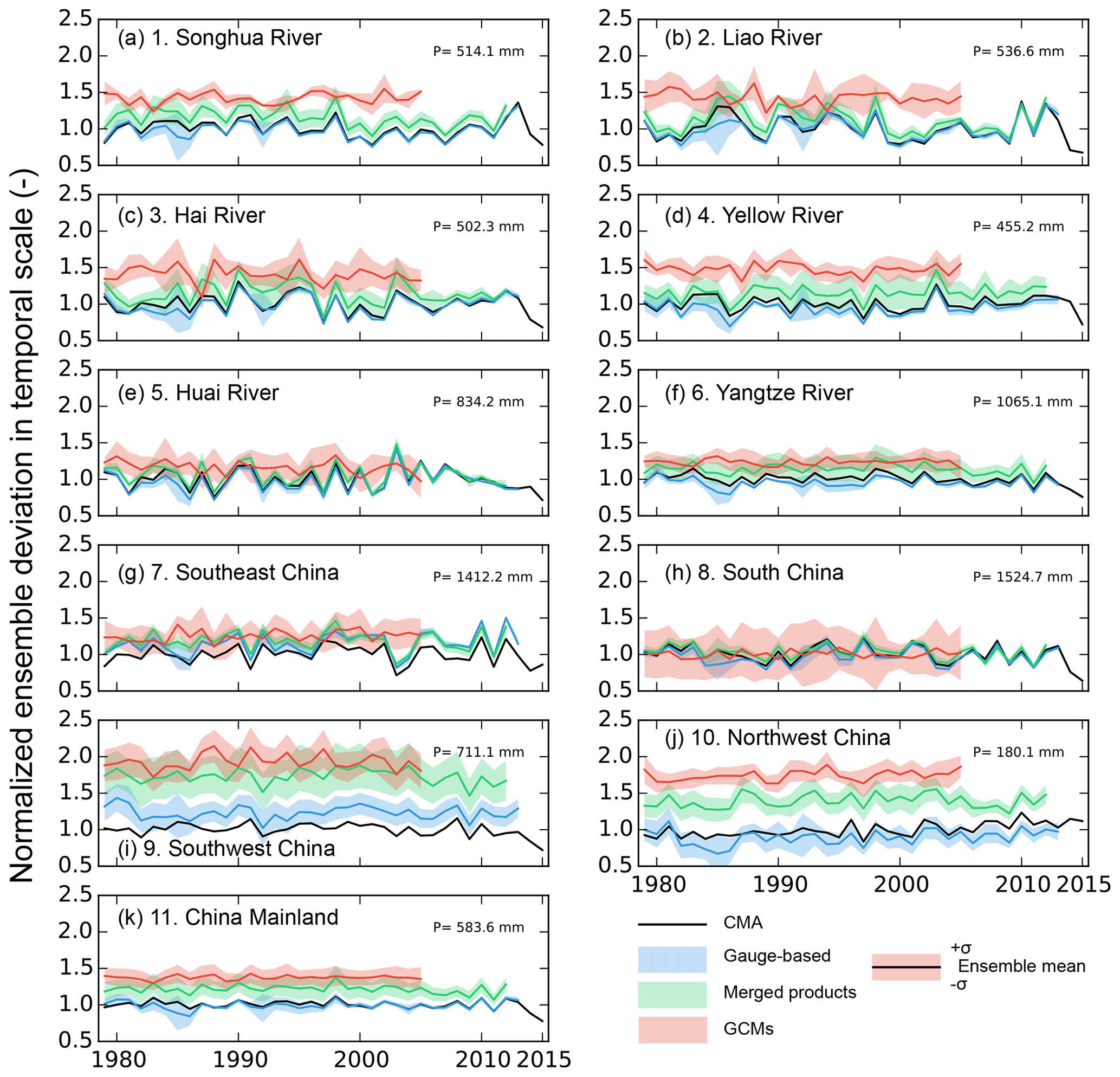
Figure 6Temporal evolution of the model uncertainty. The uncertainty is expressed as the normalized ensemble deviation of annual precipitation across ensemble datasets in each precipitation group for specific subregions. The value on the top right of each panel is the annual regional precipitation estimated in the CMA dataset (1979–2015). The annual precipitation is normalized as the ratio to the CMA long-term annual precipitation. The solid curve represents the ensemble mean of precipitation in each precipitation data group over the subregion. The width of the shaded area represents the standard deviation of the annual precipitation estimated from the datasets within that group for each year (divided by the annual precipitation of the corresponding group). The shaded area is equally distributed in the two sides of the ensemble mean values for the corresponding precipitation group.
The annual precipitation of each precipitation group has been normalized as the ratio to the long-term annual mean of the CMA in each subregion (black line in Fig. 6). The magnitude of the annual precipitation in the gauge-based products (the blue solid line) is similar to that of the CMA except in Southwest China (Fig. 6i) for the overestimation along the Himalayas (Fig. 4a, b). The precipitation in the merged products (the green solid line) is higher in Southwest and Northwest China, in accordance with Fig. 4c. The annual precipitation of the GCMs (the red solid line) is apparently higher than that of the gauge-based products and merged products for almost all regions, which agrees with the spatial patterns in Fig. 4d.
The ensemble deviation across the timescale is shown in the shaded area in Fig. 6. It is estimated as the deviation of regional annual precipitation of each product in the same group at a specific time step for each subregion. The deviation is normalized to facilitate comparisons between different subregions. High deviations are found in Southwest China (Fig. 6i) in all three precipitation groups because of the large differences along the Himalayas. The deviations of the gauge-based products and the merged products in other regions are small and getting smaller with time. This is mainly because more observations are included and technologies have improved with time to control the quality of the data. A large deviation is found in the merged products in 10-Northwest China (Fig. 6j) and 4-Yellow River Basin (Fig. 6d), where a dry climate dominates and the annual precipitation is among the lowest. The model deviation of GCMs varies between regions as it is at its smallest in 1-Songhua River Basin (Fig. 6a) and 6-Yangtze River Basin (Fig. 6f), while it is among the highest in 8-South China and West China (9, 10), agreeing with the deviation maps in Fig. 5.
Despite their mean values and magnitudes of deviation, the temporal evolutions of the gauge-based products and merged products agree well with those of the CMA dataset, while the temporal evolution of the members of the category of GCMs is weaker and not well correlated with that of the CMA. The main reason is that GCMs are not constrained in their synoptic variability and the sequence of wet and dry years can be very different from that of the observations. A smoother result is thus obtained when we build the ensemble mean from the GCMs. Unlike the weak variation in GCMs, the gauge-based and merged products have a strong co-variance, and the ensemble mean preserves this co-variance.
For the entire Chinese mainland (Fig. 6k), the ensemble deviation remains stable in different precipitation groups. In contrast, the annual precipitation spans the strongest spatial heterogeneity in the mainland compared to those divided by subregions (Fig. 4). However, the spatial variation has been collapsed because the regional precipitation has to be obtained before the temporal analysis. It is therefore interesting to evaluate how the uncertainty changes when the variations along both the time dimension and the spatial dimension are considered in the precipitation datasets.
3.4 Variations along the temporal and spatial dimensions
Previous subsections provide the deviation analysis in either temporal scale or spatial scale. However, the two are seldom compared with each other. Herein, the standard deviations of the temporal and spatial variations in the precipitation datasets are compared in Fig. 7 in 10 subregions and the China mainland for different precipitation groups. The gauge-based products provide similar annual regional precipitation to CMA over the China mainland and the 10 specific subregions except for the region 7-Southeast China (Fig. 7g) and region 9-Southwest China (Fig. 7i), while the merged products provide larger precipitation estimations for most of the regions. It might indicate the degraded ability of remote sensing, one of the important data sources in the merged products, to estimate the precipitation amount in storms as the storms mainly contribute to the total precipitation for the two subregions. The regional precipitation in GCMs is even larger except in the region 8-South China (Fig. 7h). These results indicate the degraded ability of merged products and GCMs in reproducing the total value of the annual precipitation.
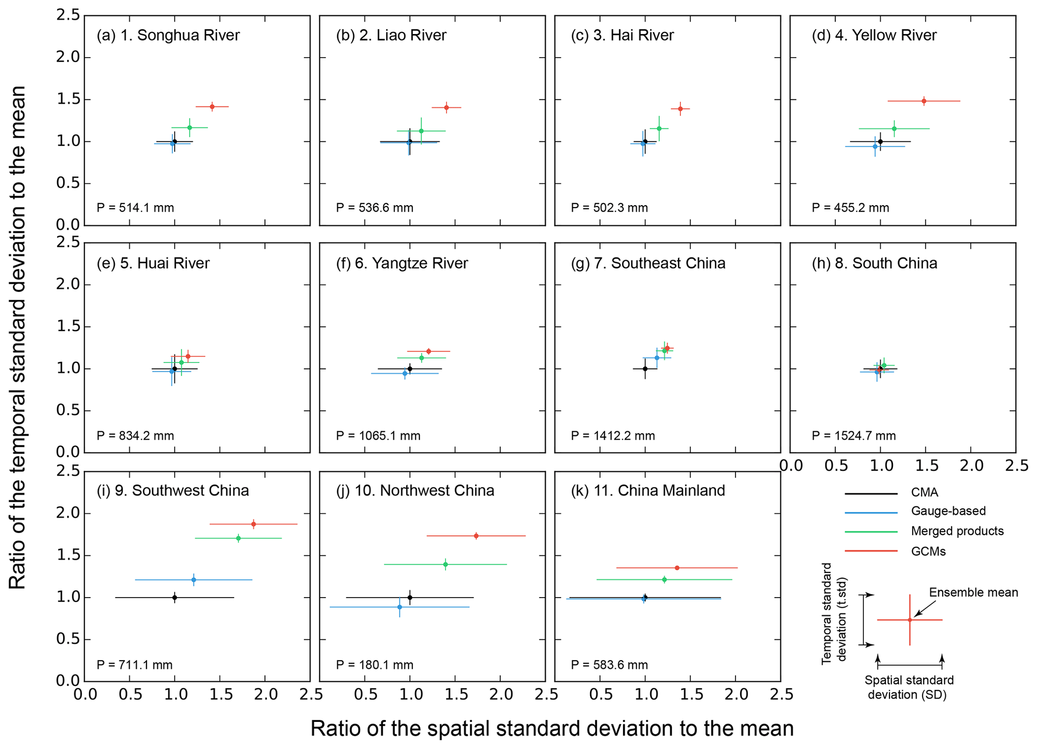
Figure 7Spatial standard deviation (horizontal) and temporal standard deviation (vertical) of the annual precipitation across ensemble datasets in each of the different precipitation groups for each subregion. The P value in the bottom left is the annual precipitation of CMA. The cross centre represents the long-term means of the regional annual precipitation in ratio to the CMA mean value. The horizontal error bar represents the spatial standard deviation (spatial variation of the long-term annual precipitation at all the grids). The vertical error bar represents the temporal standard deviation (temporal variations of region-averaged annual precipitation in different years).
The spatial standard deviations (as a ratio to the mean) in regions 9, 10 and 11 are the largest, indicating the strongest spatial heterogeneity over these regions. The smallest spatial variations are found in regions 7-Southeast China and 3-Hai River, either because of the small area or the high homogeneity in these subregions. Nevertheless, the spatial deviation in most of the subregions is larger than the temporal deviation. The ratio of the temporal deviation to the spatial deviation is among the smallest in subregions 9, 10 and 11 (k=0.1, 0.12 and 0.05, respectively; k is the ratio of the temporal deviation to the spatial deviation), showing an apparent difference between the variations along the two dimensions, while the difference between the variations along the two dimensions is small in 3-Hai River basin (k=1.15) and 7-Southeast China (k=0.90), mainly due to the relatively strong variability of the annual precipitation in different years.
In addition to the differences between regions, the variations in different precipitation groups also vary in magnitude. Excluding the CMA dataset, which consists of only one single product, the total variation (the sum of the spatial and temporal variations) across the gauge-based products is higher than that of the other two groups. This difference demonstrates that the gauge-based products may have the largest spatial variation, and the correlations between the different gauge-based products are high, so that this variation is preserved when passing to the ensemble. In contrast, variations across the GCMs are the smallest, either because the precipitation estimated in the GCMs is more spatially homogenous than that of other precipitation products or because the precipitation estimations in different GCMs are not consistent in time or space since there are no constraints on the GCM simulation. The inconsistent precipitation patterns will be further eliminated when carrying out an ensemble averaging over multiple datasets.
4.1 Variances in three dimensions
In the preceding section, we introduced the spatial and temporal characteristics of the annual precipitation. The variations in the precipitation in two dimensions of the precipitation products in the same precipitation group were estimated by two classic metrics. In this section, we will present the uncertainty results estimated by the newly proposed approach to the variance. As introduced in the Methods section, the input annual precipitation to the approach is re-organized into three dimensions: (1) time, 27 years from 1979 to 2005, (2) space, 0.5∘ grids in a specific region, and (3) ensemble, the number of models in each precipitation group (four models for each of the three groups). Note that the estimated variance is for a specific subregion because it is an analysis based on regions and a long-term scale.
The grand variance (V, total value of the variance for all three dimensions) and its three components (i.e. variance in time Vt, space Vs and ensemble dimension Ve) for all the subregions is mapped in Fig. 8. The grand variance is similar in space in groups of the gauge-based products and the merged products (Fig. 8a, b, c), while the grand variance in the GCMs is larger and is approximately twice the V in the other two groups in regions 9-South China and 10-Southwest China. The differences are mainly constituted by the spatial variance and ensemble variance (Fig. 8i, l).

Figure 8Maps of the estimated grand variance (V) and variances in different dimensions (Vt, Vs, Ve) across the ensemble datasets in each of the three different precipitation groups.
The temporal variance Vt is the smallest among all three variances, and it has very little differences in North China (Fig. 8d, e, f). But it is higher in the gauge-based products than in the merged products and GCMs in regions 8-Southeast China and 9-South China, indicating a relatively strong temporal variation in the annual precipitation series, in accordance with the larger uncertainty ranges shown in Fig. 6h, i. Similar patterns of the spatial variance Vs are found in the gauge-based products and merged products (Fig. 8g, h). The largest Vs is found in regions 7-Southeast River basin and 9-Southwest China because the precipitation significantly varies in space in these two subregions: it is higher in GCM precipitation especially in 9-Southwest China, indicating the strong spatial heterogeneity in the GCM models over the Himalayas (Fig. 8i). The ensemble variance Ve is relatively small in most regions for gauge-based products (Fig. 8j), indicating that the model variation across datasets in the observation group is small. A similarly small Ve is found in the northern regions of the merged products as well as in the GCMs for the regions in North China, while the intra-ensemble variations are large in the GCMs, especially in the south, especially 9-Southwest China and 8-South China (Fig. 8k, l).
One can conclude that the grand variance and individual variance for each of the three different dimensions are generally larger in the precipitation group consisting of GCMs. The variations for the gauge-based products and merged products are similar in values and spatial distribution. However, in addition to the variances, the deviation defined as the ratio of the square root of the variance to the mean (e.g. U, Ut, Us, Ue) contains extra information about the regional means and will be discussed in the following section.
4.2 Deviations in three dimensions
In contrast to the spatial gradient of the magnitude of the variance distributed over the 10 subregions (Fig. 8), the larger values of the total deviation () occur in the northwest, but a lower value generally occurs in South China (Fig. 9). The decreasing tendency of magnitude of the precipitation from the southeast to the northwest results in a shift of the spatial gradient compared to Fig. 4. The total deviation U is highest in Northwest China (U=0.89, Fig. 9a, b, c) for all three precipitation groups, but is relatively small in the northeastern 1-Songhua River (U=0.27) and 8-South China (U=0.29) for the gauge-based products. A relatively lower U is found in subregion 6-Yangtze River in the merged products and GCMs in the eastern part of China.
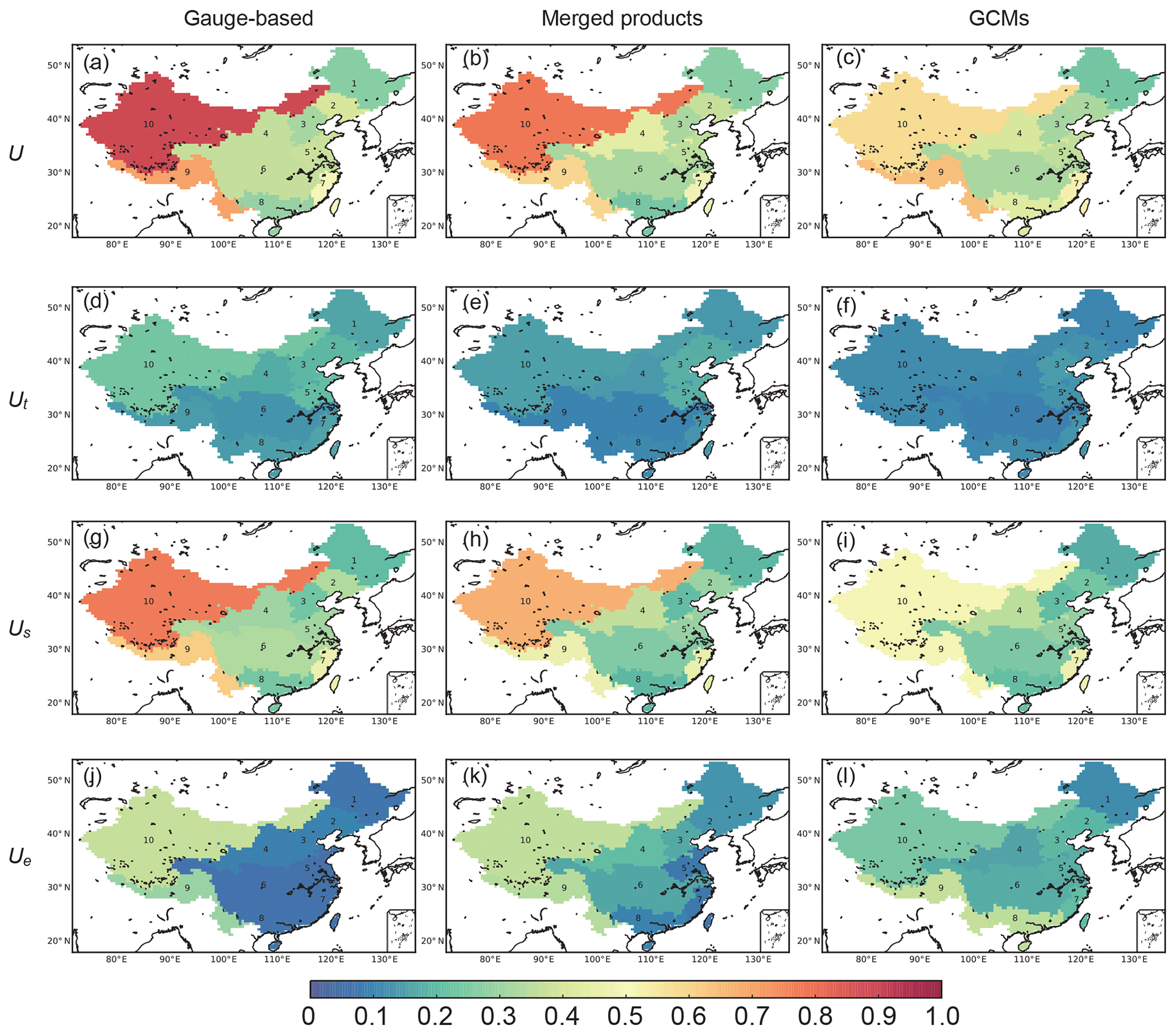
Figure 9Maps of deviations (U, Ut, Us, Ue) estimated as the ratio of the square root of the corresponding variances (i.e. V, Vt, Vs, Ve) to the regional mean (μ) of the ensemble datasets in each of the three different precipitation groups. Of these, Ue is considered to be the model uncertainty.
Deviations along the temporal and spatial dimensions are inherent, as they show the temporal evolution and spatial heterogeneity of the precipitation products. The results show that Ut is small and contributes very little to the total U, indicating the weak fluctuation of annual precipitation compared to the spatial heterogeneity (Fig. 9d, e, f). The smallest value of Ut for the GCMs is in accordance with the weakest temporal variations in Fig. 6. The deviation in the spatial dimension (Us) contributes the most to the total deviation, especially in Northwest China (Us=0.77 for the gauge-based products, Fig. 9g). The high Us indicates the strong spatial heterogeneity of precipitation in the region, demonstrating that the ability to describe the precipitation varies significantly in different places in the subregions. However, because the spatial variations obtained by the GCMs in Northwest China are less significant than with the other two groups, the value of Us for region 10-Southwest China (=0.51) is smaller than that of the gauge-based and merged products.
The variations along the temporal and spatial dimensions show the natural precipitation patterns, but the deviation of multiple products (Ue) shows the ability to consistently represent the spatiotemporal patterns. Therefore, Ue indicates the uncertainty of the ensemble precipitation products in the same group. For the gauge-based products, Ue is smaller than 0.1 for regions in East China, indicating that the model variations are relatively small compared to the annual means. The value of Ue is higher for 9-Southwest China (=0.30) and 10-Northwest China (=0.37), showing large variations even in the gauge-based products. For the merged products, Ue is similar to that of the gauge-based products in West China (=0.36), while it is larger in the east, especially for 6-Yangtze River and 4-Yellow River (more than 2 times larger than Ue of the gauge-based products).
For the GCM precipitation, Ue increases compared to the other two groups in the eastern subregions, corresponding to the higher spatial model uncertainty in GCMs over the eastern regions shown in Fig. 5. It decreases in 10-Northwest China (Ue=0.25), and a possible reason for this is that the spatial homogeneity of the variations in 10-Northwest China (Fig. 5f) is stronger than that of the other groups (Fig. 5b, d, f). In the GCMs, the highest Ue occurs in Southwest China, where both the means and the variations are higher (Figs. 4 and 5). One can conclude that Ue is linked with the magnitude of the model uncertainties in Figs. 5 and 6, indicating that it is to some degree correlated with the classic metrics, as higher Ue covers the grid cells or regions with higher model uncertainty.
5.1 Deviation from the classic uncertainty metrics
In this section, we will compare the uncertainty Ue of the ensemble members estimated by the three-dimensional partitioning approach with the two classic metrics defined as N.s.std in Eq. (28) and N.t.std in Eq. (29), to explain how these three metrics are related and differ with each other. As shown in Fig. 10, Ue is correlated with both N.s.std and N.t.std. The correlation is stronger when Ue is smaller than 0.2, where the regions from 1 to 8 are generally included for all three precipitation groups. But Ue is in general larger than N.s.std and N.t.std for the products. This deviation is because the variation along one dimension has been collapsed when calculating the deviation along the other dimension. For subregions 9, 10 and 11, N.s.std and N.t.std deviate the most from the 1:1 line of Ue. Taking subregion 9-Southwest China in the gauge-based products as an example, the temporal variance is 62.4 mm yr−1, while the spatial variance is 571.8 mm yr−1 (Fig. 7i). The difference between N.s.std and Ue is 0.058 (=0.297–0.239; the deviation ratio is 24.3 %) when the temporal variation is collapsed. The difference between N.t.std and Ue is 0.126 (=0.297–0.171; the deviation ratio is 73.4 %) when the spatial variation is collapsed. The deviation is significantly larger than that between Ue and N.s.std, showing that the collapse will induce a deviation related to the magnitude of the collapsed dimension.
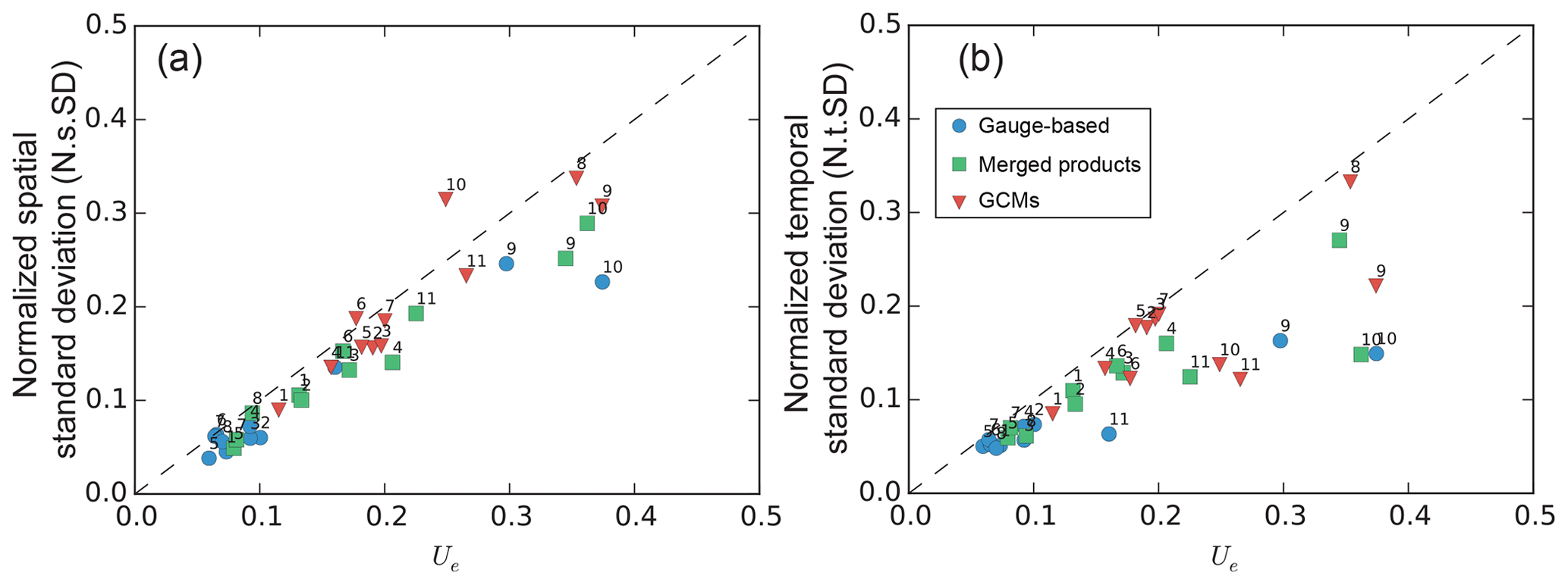
These subregions (9, 10, 11) feature strong spatial heterogeneities (Fig. 7i, j, k) in the annual mean precipitation (Fig. 4). The averaging process before estimating the classic metrics will cause a significant smoothing of the datasets when the spatial heterogeneity of the datasets is very strong, because the spatial variation is significantly higher than the temporal variation, as shown in Fig. 7. The estimation of N.t.std, which needs an averaging over the spatial dimension, will lose more information than that in the time dimension. The deviation between N.t.std and Ue (Fig. 10b) is larger than that between N.s.std and Ue (Fig. 10a). The priority of the precipitation types also changes, from model dominated (the model uncertainties in GCMs are larger than the others) to region dominated (the uncertainties in the specific regions 9, 10, and 11 are larger than in the other regions no matter which precipitation data are used). This indicates that the difference in model variation over space can be reflected in the new uncertainty Ue.
Each classic metric has its physical meaning: N.s.std represents the uncertainties over space and N.t.std represents the uncertainties across time. The comparison of Ue with each of them demonstrates the metric performance on the same physical meaning. It is possible to compare Ue with a combination of the two classic metrics, but the combination could be far more complex than a simple sum of the two classic metrics. However, a qualitative comparison is accessible because Ue has a linear correlation with either of them. This correlation will persist and occur between Ue and a combination of the two classic metrics by summing them up with certain weights.
5.2 Decomposition of the ensemble uncertainty
We now decompose the ensemble variance to determine the reason for the deviation of Ue from N.s.std and N.t.std. As shown in Eq. (26), the ensemble variance Ve is expressed by
This combines four components which stand for the variation of different estimates across the ensemble dimension (i.e. the variance of original temporal and spatial values, , of the temporal mean, , of the spatial mean, , and of the grand mean, ). Among these, is the mean of the squares of the spatial deviation in Fig. 5a, c, e for all grids in a specific region and is the mean of the squares of the temporal deviation in Fig. 6 for each time step in a specific region. These two components are closely related to the two classic metrics N.s.std (Eq. 28) and N.t.std (Eq. 29), respectively.
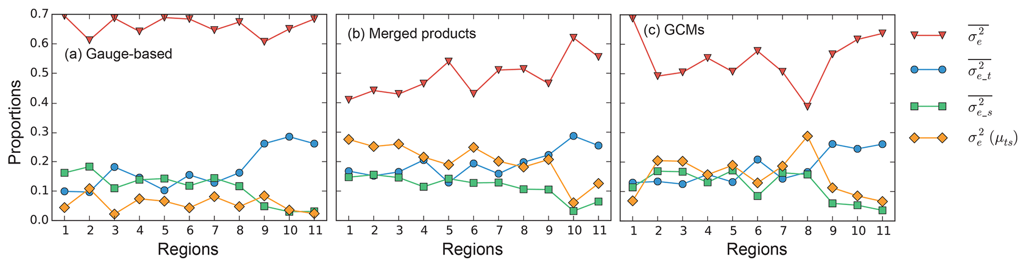
Figure 11Proportions of the four components in Eq. (30) to Ve of the ensemble datasets in each of the three different precipitation groups: (a) gauge-based products, (b) merged products and (c) GCMs. The contribution is normalized so that their sum is 1.0 for each region. Among the four components, and are associated with the two classic metrics N.s.std and N.t.std, respectively.
By decomposing Eq. (30), the contributions of the four components to the ensemble variance Ve are shown in Fig. 11. For all three precipitation groups, is the dominant component simply because all the information on variations of the original datasets is retained in the uncertainty estimation. The other three components result from estimations after an averaging is performed, either over time, space, or the full spatiotemporal dimensions, which means a loss of information. The contribution of and approximates 0.15 for the regions from 1 to 8. But increases for regions 9, 10 and 11, indicating that there is significant spatial heterogeneity in these regions. In contrast, decreases because the spatial averaging has collapsed the spatial variations. The very small contribution of related to N.t.std is the cause of larger deviations between N.t.std and Ue in these subregions (Fig. 10b).
Although any component can be used as a metric for evaluating the variations of multiple datasets, there are limitations for each of the variations. Regarding the variation of the temporal mean and spatial mean , the collapse of a dimension has ignored part of the information. Moreover, the variation of the grand mean has ignored both the temporal variability and spatial heterogeneity, which further decreases its applicability to the assessment of uncertainty. The variation is estimated based on the original data without averaging, and thus it represents the most information. However, it does not take into account the systematic uncertainty (bias in the mean values) which is expressed by .
Therefore, none of the single components is able to represent the others. The integrated metric Ve is therefore a solution that represents all metrics to different degrees. What is interesting is that the variability of the proportions of and (or and ) are opposite and the sum of their proportions is stable, around 0.3 (or 0.7). This indicates a complementary relation between the two pairs of elements ( and ; and ). On the other hand, some of the information is ignored in one of the components but remains in the other one within the same pair. Therefore, the variation along the time dimension and that along the spatial dimension should be considered together, as is done in the estimation of the ensemble variance Ve. The normalized uncertainty Ue derived from the integrated variation Ve, which is better able to determine the uncertainties than are the classic metrics, should be the more proper choice for an uncertainty analysis.

5.3 Differences between the metrics in value and proportion
Figure 10 shows that Ue is generally higher than the uncertainty identified by the two classic metrics (i.e. N.s.std and N.t.std). Figure 12 then summarizes the magnitude of the deviations of the classic metrics from the new uncertainty Ue. We can see that the two classic metrics generally underestimate the uncertainty by around 0.03 (Fig. 12a). The variation of the underestimation of N.t.std is larger than that of N.s.std, showing a larger deviation between Ue and N.t.std. Employing the new uncertainty metric will increase the estimated uncertainty by around 20 %–40 % for half of the cases, when compared to N.s.std (Fig. 12b). For nearly 25 % of the cases, the new Ue increases the estimated uncertainty by more than 50 %. In extreme cases, Ue is more than double N.t.std (Fig. 12b). The results show that the widely applied uncertainty estimates from the two classic metrics have underestimated the uncertainty of the various models or datasets. Such an underestimation may especially occur for the temporal assessment of the uncertainties (N.t.std), which is very commonly seen in scientific reports and articles to illustrate the temporal evolution of the variables of interest.
6.1 Features and applicability of the approach
The total variation across the database which consists of multiple datasets is contributed by the spatiotemporal variations as well as the uncertainties of ensemble datasets, while the uncertainty assessment with current approaches (e.g. Eqs. 28 and 29) needs either the temporal variability or the spatial heterogeneity to be averaged, which means a loss of information. The variance partitioning approach proposed in this study works in three dimensions. It uses all the information over both the temporal and spatial dimensions of the multiple ensemble members. It avoids the collapse of variation along any dimension, and thus the proposed uncertainty estimate Ue provides a more accurate estimate of the uncertainty. The estimate Ue is especially suitable for an overall assessment of the multiple datasets over a certain period and over a specific space. Even though the trade-off is that Ue cannot provide the temporal evolution or spatial heterogeneity for users' consideration, in many cases we would like to know the general performance of the ensemble models based on a global single estimate.
The results of this partitioning approach can be affected by the choice of the time step intervals. For example, the temporal variance or proportion of temporal variance will significantly increase if the time interval is chosen to be 1 month. The intra-annual variability of precipitation will result in higher Vt. The changes depend on how significant the intra-annual variability is compared to the inter-annual variations. Moreover, only changes in the temporal variation (the average values remain but the magnitudes of the variation increase or decrease) can be captured by Ue. But N.s.std will remain the same because the temporal variability has been neglected in the averaging process. It is the same with N.t.std if different spatial resolutions of the measurements are used.
The proposed approach has a flexible structure that can deal with different problems, from a global scale to regional studies. The temporal dimension can also span from daily, monthly, annual to decadal analyses with different scopes. The ensemble dimension is applicable from two members (i.e. model evaluation between simulations and observations) to any number of multi-models (consensus evaluation, Tebaldi et al., 2011; McSweeney and Jones, 2013). The present approach is also applicable to any variables that can be organized into three dimensions, such as climatic variables (e.g. temperature, evaporation), hydrological variables (e.g. soil moisture, runoff) or environmental variables (e.g. drought index). Based on these advantages, this three-dimensional partitioning approach can be widely applied in hydro-climatic analysis.
6.2 Conclusions
A new three-dimensional partitioning approach has been proposed in this paper to assess the model uncertainties of multiple ensemble datasets. The new uncertainty metric (Ue) is estimated with an overall consideration of temporal and spatial variations as well as the differences among the ensemble products. The results have shown that Ue is generally larger than the classic uncertainty metrics N.s.std and N.t.std, which require a collapse of the variation along either the temporal or spatial dimension. The deviation occurs where the spatial variations are significant but being averaged in the N.t.std estimation. The decomposition of the total variance Ve shows the complementary relation between the two classic metrics, and therefore the new uncertainty Ue (derived from Ve) is a more comprehensive estimate of the uncertainty of multiple ensemble products.
Thirteen precipitation datasets generated by different methods have been categorized into three groups (namely, gauge-based products, merged products and GCMs) and the model uncertainty in the ensemble products has been analysed with the new approach and with the two classic uncertainty metrics for each precipitation group. Using the classic metrics, in most regions, uncertainty of GCMs has been found to be the largest. But the new estimator Ue indicates that the largest model uncertainty occurs in specific regions no matter which precipitation group is considered. The impact of spatial heterogeneity on the model uncertainty has been represented well in the new uncertainty metric (Ue). In addition to the theoretical analysis of the components of Ue, the overall model uncertainty Ue can be used as a new uncertainty estimate which involves more information and should receive more attention in the field of uncertainty assessment.
Zone A:
A1:
A2:
A3:
Zone B:
B1:
B2:
B3:
Zone C:
C1:
C2:
C3:
C4:
C5:
C6:
Zone D:
D1:
D2:
D3:
Zone E:
E1:
E2:
E3:
Zone F:
F1:
F2:
F3:
The t, s, and e in the algorithms represent the three dimensions time, space and ensemble, with the sizes of m,n, and l and index with i,j, and k, respectively.
Each expression is shown with its size and the meaning of each dimension.
For example, for A1, , the μt has a size of n×l.
The first axis represents the space dimension, and the second is the ensemble dimension, while C1 () has only one ensemble dimension with its size as l.
F1 () is only a single value.
The CMA dataset is available through http://data.cma.cn/data/detail/dataCode/SEVP_CLI_CHN_ PRE_DAY_GRID_0.50/ (Zhao et al., 2018). The GPCC is available through https://opendata.dwd.de/climate_environment/GPCC/html/fulldata_v6_doi_download.html (Schneider et al., 2011). The CRU is available through https://iridl.ldeo.columbia.edu/SOURCES/.UEA/.CRU/.TS3p21/ (Harris et al., 2014). The CPC is available through http://ftp.cpc.ncep.noaa.gov/precip/CPC_UNI_PRCP/ (Xie et al., 2007). The UDEL is available through http://climate.udel.edu/data (Willmott and Matsuura, 2012). The CMAP is available through https://www.esrl.noaa.gov/psd/data/gridded/data.cmap.html (Xie et al., 2003). The GPCP is available through https://www.esrl.noaa.gov/psd/data/gridded/data.gpcp.html (Adler et al., 2018). The MSWEP is available through https://platform.princetonclimate.com/PCA_ Platform/mswepRetro.html (Beck et al., 2017). The ERA-I is available through https://www.ecmwf.int/en/forecasts/datasets/reanalysis-datasets/era-interim/ (Dee et al., 2011). The GCMs (including HadCM3, IPSL-CM5A-LR, CMCC-CM and MIROC5) are available through https://esgf-node.llnl.gov/projects/cmip5/ (Taylor et al., 2012).
XZ initialized the ideas presented in this paper with supervision from JP and TY. XZ prepared the simulations, the figures and the manuscript. CSH participated in the data preparation. All the authors contributed to the discussion and revising the paper.
The authors declare that they have no conflict of interest.
The work was supported by computing resources of the IPSL ClimServ cluster at the École Polytechnique, France.
This research has been supported by the National Natural Science Foundation of China (grant nos. 41561134016 and 51879068), the ANR (grant no. ANR-15-CE01-00L1-0L), the National Key Research and Development Program (grant no. 2018YFC0407900), and the China Scholarship Council (grant no. 201506710042).
This paper was edited by Dimitri Solomatine and reviewed by two anonymous referees.
Adler, R. F., Sapiano, M. R., Huffman, G. J., Wang, J. J., Gu, G., Bolvin, D., Chiu, L., Schneider, U., Becker, A., Nelkin, E., Xie, P., Ferraro, R., and Shin, D. B.: The Global Precipitation Climatology Project (GPCP) monthly analysis (New Version 2.3) and a review of 2017 global precipitation, Atmosphere, 9, 138, https://doi.org/10.3390/atmos9040138, 2018 (data available at: https://www.esrl.noaa.gov/psd/data/gridded/data.gpcp.html, last access: 18 April 2020). a, b
Beck, H. E., van Dijk, A. I. J. M., Levizzani, V., Schellekens, J., Miralles, D. G., Martens, B., and de Roo, A.: MSWEP: 3-hourly 0.25∘ global gridded precipitation (1979–2015) by merging gauge, satellite, and reanalysis data, Hydrol. Earth Syst. Sci., 21, 589–615, https://doi.org/10.5194/hess-21-589-2017, 2017 (data available at: https://platform.princetonclimate.com/PCA_Platform/mswepRetro.html, last access: 18 April 2020). a, b, c
Bosshard, T., Carambia, M., Goergen, K., Kotlarski, S., Krahe, P., Zappa, M., Schär, C., and Schar, C.: Quantifying uncertainty sources in an ensemble of hydrological climate-impact projections, Water Resour. Res., 49, 1523–1536, https://doi.org/10.1029/2011WR011533, 2013. a
Dee, D. P., Uppala, S. M., Simmons, A. J., Berrisford, P., Poli, P., Kobayashi, S., Andrae, U., Balmaseda, M. A., Balsamo, G., Bauer, P., Bechtold, P., Beljaars, A. C., van de Berg, L., Bidlot, J., Bormann, N., Delsol, C., Dragani, R., Fuentes, M., Geer, A. J., Haimberger, L., Healy, S. B., Hersbach, H., Hólm, E. V., Isaksen, L., Kållberg, P., Köhler, M., Matricardi, M., Mcnally, A. P., Monge-Sanz, B. M., Morcrette, J. J., Park, B. K., Peubey, C., de Rosnay, P., Tavolato, C., Thépaut, J. N., and Vitart, F.: The ERA-Interim reanalysis: Configuration and performance of the data assimilation system, Q. J. Roy. Meteorol. Soc., 137, 553–597, https://doi.org/10.1002/qj.828, 2011 (data available at: https://www.ecmwf.int/en/forecasts/datasets/archive-datasets/reanalysis-datasets/era-interim, last access: 18 April 2020). a, b, c
Déqué, M., Rowell, D. P., Lüthi, D., Giorgi, F., Christensen, J. H., Rockel, B., Jacob, D., Kjellström, E., De Castro, M., and Van Den Hurk, B.: An intercomparison of regional climate simulations for Europe: Assessing uncertainties in model projections, Climatic Change, 81, 53–70, https://doi.org/10.1007/s10584-006-9228-x, 2007. a
Everitt, B.: The Cambridge Dictionary of Statistics, vol. 53, Cambridge University Press, https://doi.org/10.1017/CBO9781107415324.004, 2013. a
Harris, I., Jones, P. D., Osborn, T. J., and Lister, D. H.: Updated high-resolution grids of monthly climatic observations – the CRU TS3.10 Dataset, Int. J. Climatol., 34, 623–642, https://doi.org/10.1002/joc.3711, 2014 (data available at: https://iridl.ldeo.columbia.edu/SOURCES/.UEA/.CRU/.TS3p21/, last access: 18 April 2020). a, b, c
IPCC: Technical Summary, in: Climate Change 2013: The Physical Science Basis, Contribution of Working Group I to the Fifth Assess- ment Report of the Intergovernmental Panel on Climate Change, Cambridge University Press, Cambridge, United Kingdom and New York, NY, USA, 2013a. a
IPCC: Summary for Policymakers, in: Climate Change 2013: The Physical Science Basis. Contribution of Working Group I to the Fifth Assessment Report of the Intergovernmental Panel on Climate Change, Cambridge University Press, Cambridge, United Kingdom and New York, NY, USA, 2013b. a, b
Kay, J. E., Deser, C., Phillips, A., Mai, A., Hannay, C., Strand, G., Arblaster, J. M., Bates, S. C., Danabasoglu, G., Edwards, J., Holland, M., Kushner, P., Lamarque, J. F., Lawrence, D., Lindsay, K., Middleton, A., Munoz, E., Neale, R., Oleson, K., Polvani, L., and Vertenstein, M.: The community earth system model (CESM) large ensemble project: A community resource for studying climate change in the presence of internal climate variability, B. Am. Meteorol. Soc., 96, 1333–1349, https://doi.org/10.1175/BAMS-D-13-00255.1, 2015. a, b
Kottek, M., Grieser, J., Beck, C., Rudolf, B., and Rubel, F.: World map of the Köppen-Geiger climate classification updated, Meteorol. Z., 15, 259–263, https://doi.org/10.1127/0941-2948/2006/0130, 2006. a
Landerer, F. W. and Swenson, S. C.: Accuracy of scaled GRACE terrestrial water storage estimates, Water Resour. Res., 48, 1–11, https://doi.org/10.1029/2011WR011453, 2012. a
McSweeney, C. F. and Jones, R. G.: No consensus on consensus: The challenge of finding a universal approach to measuring and mapping ensemble consistency in GCM projections, Climatic Change, 119, 617–629, https://doi.org/10.1007/s10584-013-0781-9, 2013. a
Menne, M. J., Durre, I., Vose, R. S., Gleason, B. E., and Houston, T. G.: An overview of the global historical climatology network-daily database, J. Atmos. Ocean. Tech., 29, 897–910, https://doi.org/10.1175/JTECH-D-11-00103.1, 2012. a
Phillips, T. J. and Gleckler, P. J.: Evaluation of continental precipitation in 20th century climate simulations: The utility of multimodel statistics, Water Resour. Res, 42, 1–10, https://doi.org/10.1029/2005WR004313, 2006. a
Rodell, M., Houser, P., Jambor, U., Gottschalck, J., Mitchell, K., Meng, C.-J., Arsenault, K., Cosgrove, B., Radarkovich, J., Bosilovich, M., Entin, J., Walker, J., Lohmann, D., and Toll, D.: The Global Land Data Assimilation System, B. Am. Meteorol. Soc., 44, 381–394, https://doi.org/10.1175/BAMS-85-3-381, 2004. a
Schewe, J., Heinke, J., Gerten, D., Haddeland, I., Arnell, N. W., Clark, D. B., Dankers, R., Eisner, S., Fekete, B. M., Colón-González, F. J., Gosling, S. N., Kim, H., Liu, X., Masaki, Y., Portmann, F. T., Satoh, Y., Stacke, T., Tang, Q., Wada, Y., Wisser, D., Albrecht, T., Frieler, K., Piontek, F., Warszawski, L., and Kabat, P.: Multimodel assessment of water scarcity under climate change, P. Natl. Acad. Sci. USA, 111, 3245–3250, https://doi.org/10.1073/pnas.1222460110, 2014. a
Schneider, U., Becker, A., Finger, P., Meyer-Christoffer, A., Rudolf, B., and Ziese, M.: GPCC Full Data Reanalysis Version 6.0 at 0.5∘: Monthly Land-Surface Precipitation from Rain-Gauges built on GTS-based and Historic Data, https://doi.org/10.5676/DWD_GPCC/FD_M_V6_050 (data available at: https://opendata.dwd.de/climate_environment/GPCC/html/fulldata_v6_doi_download.html, last access: 18 April 2020), 2011. a, b
Sun, F., Roderick, M. L., Farquhar, G. D., Lim, W. H., Zhang, Y., Bennett, N., and Roxburgh, S. H.: Partitioning the variance between space and time, Geophys. Res. Lett., 37, L12704, https://doi.org/10.1029/2010GL043323, 2010. a
Sun, F., Roderick, M. L., and Farquhar, G. D.: Changes in the variability of global land precipitation, Geophys. Res. Lett., 39, L19402, https://doi.org/10.1029/2012GL053369, 2012. a
Sun, Q., Miao, C., Duan, Q., Ashouri, H., Sorooshian, S., and Hsu, K. L.: A Review of Global Precipitation Data Sets: Data Sources, Estimation, and Intercomparisons, Rev. Geophys., 56, 79–107, https://doi.org/10.1002/2017RG000574, 2018. a
Tapiador, F. J., Turk, F. J., Petersen, W., Hou, A. Y., Garcia-Ortega, E., Machado, L. A. T., Angelis, C. F., Salio, P., Kidd, C., Huffman, G. J., and de Castro, M.: Global precipitation measurement: Methods, datasets and applications, Atmos. Res., 104–105, 70–97, https://doi.org/10.1016/j.atmosres.2011.10.021, 2012. a
Taylor, K. E., Stouffer, R. J., and Meehl, G. A.: An overview of CMIP5 and the experiment design, B. Am. Meteorol. Soc., 93, 485–498, https://doi.org/10.1175/bams-d-11-00094.1, 2012 (data available at: https://esgf-node.llnl.gov/projects/cmip5/, last access: 18 April 2020). a
Tebaldi, C., Arblaster, J. M., and Knutti, R.: Mapping model agreement on future climate projections, Geophys. Res. Lett., 38, L23701, https://doi.org/10.1029/2011GL049863, 2011. a
Willmott, C. J. and Matsuura, K.: Terrestrial Air Temperature and Precipitation: Monthly and Annual Time Series (1900–2010), 2012 (data available at: http://climate.udel.edu/data, last access: 18 April 2020). a, b
Xie, P., Janowiak, J. E., Arkin, P. A., Adler, R., Gruber, A., Ferraro, R., Huffman, G. J., and Curtis, S.: GPCP pentad precipitation analyses: An experimental dataset based on gauge observations and satellite estimates, J. Climate, 16, 2197–2214, https://doi.org/10.1175/2769.1, 2003 (data available at: https://www.esrl.noaa.gov/psd/data/gridded/data.cmap.html, last access: 18 April 2020). a, b
Xie, P., Chen, M., Yang, S., Yatagai, A., Hayasaka, T., Fukushima, Y., and Liu, C.: A Gauge-Based Analysis of Daily Precipitation over East Asia, J. Hydrometeorol., 8, 607–626, https://doi.org/10.1175/JHM583.1, 2007 (data available at: http://ftp.cpc.ncep.noaa.gov/precip/CPC_UNI_PRCP/, last access: 18 April 2020). a, b
Zhao, Y., Zhu, J., Xu, Y., and Liu, N.: Monthly gridded surface precipitation at 0.5∘ in China (V2.0), National Meteorological Information Center, China, 2018 (data available at: http://data.cma.cn/data/detail/dataCode/SEVP_CLI_CHN_PRE_DAY_GRID_0.50/, last access: 18 April 2020). a, b
- Abstract
- Introduction
- Method and datasets
- Characteristics of precipitation and model-quantified uncertainties with classic metrics
- Variances in precipitation products
- Comparison of the uncertainty Ue with the classic metrics
- Discussion and conclusions
- Appendix A: The algorithms for different expressions in the methodology
- Data availability
- Author contributions
- Competing interests
- Acknowledgements
- Financial support
- Review statement
- References