the Creative Commons Attribution 4.0 License.
the Creative Commons Attribution 4.0 License.
 | 16 Jan 2020
Assessing the perturbations of the hydrogeological regime in sloping fens due to roads
Fabien Cochand
Daniel Käser
Philippe Grosvernier
Daniel Hunkeler
Roads in sloping fens constitute a hydraulic barrier for surface and subsurface flow. This can lead to the drying out of downslope areas of the sloping fen as well as gully erosion. Different types of road construction have been proposed to limit the negative implications of roads on flow dynamics. However, so far, no systematic analysis of their effectiveness has been carried out. This study presents an assessment of the hydrogeological impact of three types of road structures in semi-alpine, sloping fens in Switzerland. Our analysis is based on a combination of field measurements and fully integrated, physically based modeling. In the field approach, the influence of roads was examined using tracer tests in which the area upslope of the road was sprinkled with a saline solution. The spatial distribution of electrical conductivity downslope provided a qualitative assessment of the flow paths and, thus, the implications of the road structures on subsurface flow. A quantitative albeit not site-specific assessment was carried out using fully coupled numerical models jointly simulating surface and subsurface flow processes. The different road types were implemented and their influence on flow dynamics was assessed for a wide range of slopes and different hydraulic conductivities of the soil. The models are based on homogenous soil conditions, allowing for a relative ranking of the impact of the road types. For all cases analyzed in the field and simulated using the numerical models, roads designed with an L drain (i.e., collecting water upslope and releasing it in a concentrated manner downslope) constitute the largest perturbations in terms of flow dynamics. The other road structures investigated were found to have less impact. The developed methodologies and results can be used for the planning of future road projects in sloping fens.


Wetlands can play a significant role in flood control (Baker et al., 2009; Zollner, 2003; Reckendorfer et al., 2013), mitigate climate change impacts (Cognard Plancq et al., 2004; Samaritani et al., 2011; Lindsay, 2010; Limpens et al., 2008), and feature great biodiversity (Rydin and Jeglum, 2005). However, the world has lost 64 % of its wetland areas since 1900 and an even greater loss has been observed in Switzerland (Broggi, 1990). Therefore, wetland conservation has received considerable attention. However, the sprawl of human infrastructure, land use change, climate change, and river regulation remain serious factors that threaten wetlands. For instance, roads can substantially modify the surface–subsurface flow patterns of sloping fens. These changes in flow patterns can influence sediment transport, moisture dynamics, and biogeochemical processes as well as ecological dynamics.
The link between hydrological changes and sediment dynamics has been studied in various contexts (see, e.g., Partington et al., 2017). From a civil engineering perspective, erosion of the road must be avoided. A common strategy to avoid erosion of the road foundation is to collect water in drains and then release it in a concentrated manner downslope. This, however, can lead to erosion of the downslope area, a phenomenon known as “gully erosion”. A number of studies have specifically focused on identifying the controlling processes and relevant parameters of gully erosion (Capra et al., 2009; Valentin et al., 2005; Descroix et al., 2008; Poesen et al., 2003; Martínez-Casasnovas, 2003; Daba et al., 2003; Betts and DeRose, 1999; Derose et al., 1998). Nyssen et al. (2002) investigated the impact of road construction on gully erosion in the northern Ethiopian highlands, with a focus on surface water. In their study area, they observed the formation of a gully downslope of the outlets of the drains after the road construction. Based on fieldwork and subsequent statistical analysis, they concluded that the main causes of gully development are concentrated runoff, the diversion of concentrated runoff to other catchments, and the modifications of drainage areas induced by the road. The role of groundwater was not considered in this study.
Reid and Dunne (1984) developed an empirical model for estimating road sediment erosion of roads located in forested catchments in Washington state, USA. They concluded that a heavily used road produced 130 times more sediment than an abandoned road. Wemple and Jones (2003) also developed an empirical model for estimating the runoff production of a forest road at the catchment scale. They demonstrated that during large storm events, subsurface flow can be intercepted by the road. The intercepted water, if directly routed to ditches, increases the rising limb of the catchment hydrograph. At a smaller spatial scale (0.1 km2), Loague and VanderKwaak (2002) assessed the impact of a road on the surface and subsurface flow using the InHM (Integrated Hydrology Model) integrated surface–subsurface flow model (VanderKwaak, 1999) in a rural catchment. The results showed that the road induced a slight increase in runoff and a decrease in surface–subsurface water exchange around the road. Dutton et al. (2005) investigated the impact of roads on the near-surface subsurface flow using a variability saturated subsurface model. They concluded that the permeability contrast caused by the road construction leads to a disturbance of near-surface subsurface flow which may significantly modify the physical and ecological environment.
Road construction can also impact the development of vegetation (Chimner et al., 2016). Von Sengbusch (2015) investigated changes in the growth of bog pines located in a mountain mire in the black forest (southwest Germany). The author suggested that the increase in bog pine cover was caused by a delayed effect from road construction in 1983 along a margin of the bog. The road affected the subsurface flow and therefore prevented the upslope water from flowing to the bog. According to von Sengbusch (2015), road disturbances induce a larger variability in water table elevations during dry periods and consequently increase the sensitivity of the bog to climate change.
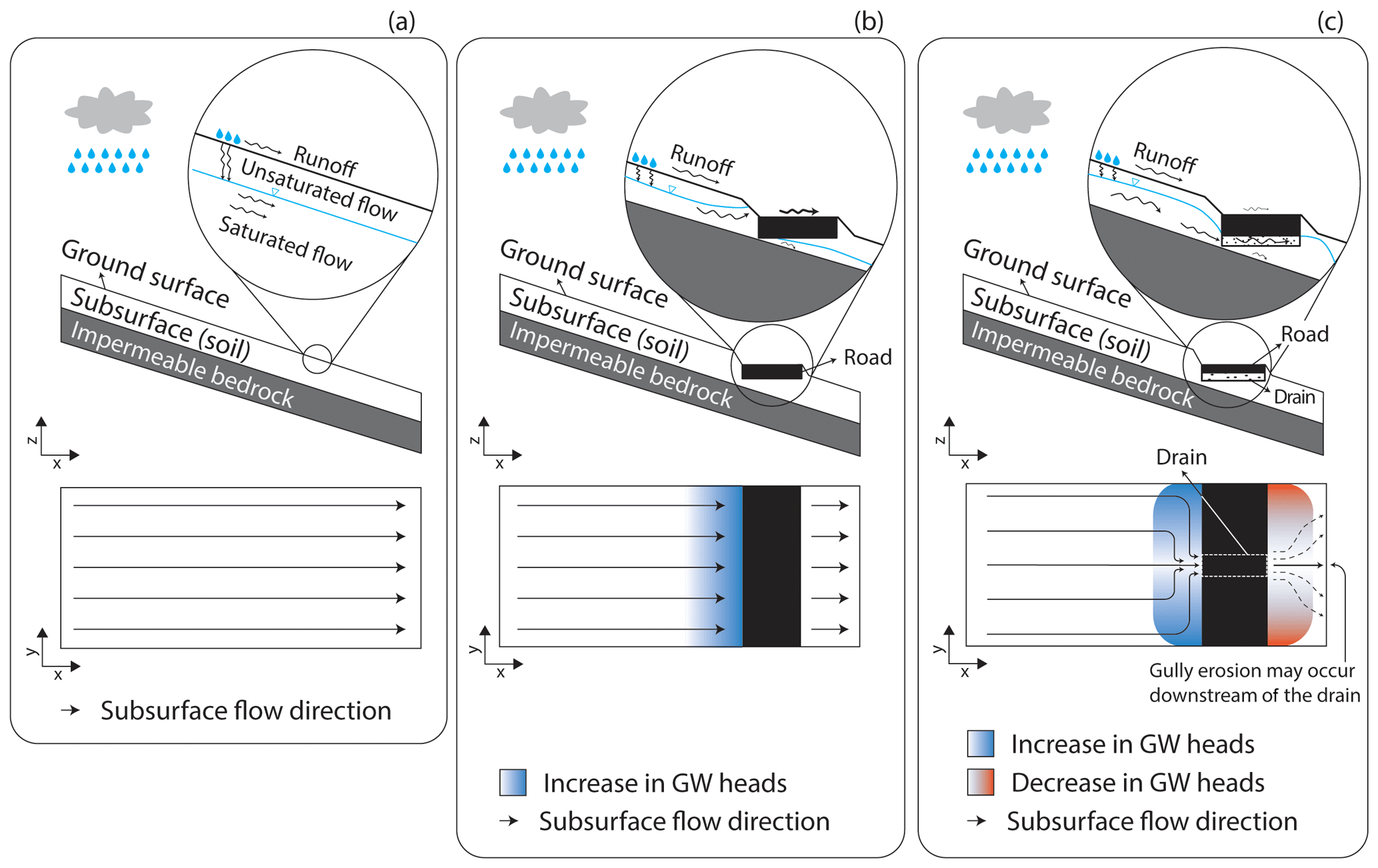
Figure 1Conceptual subsurface dynamics in sloping fens. (a) Natural conditions. (b) A road without a drain (only shown for illustrative purposes as essentially all roads have drains); in this case, water will flow both across and under the road. Uncontrolled flow beneath the road can cause erosion of the road foundation. (c) A road with a drain; in this design, surface water flow is reduced and flow beneath the road occurs in a controlled manner through the drain. Water is released downslope in a concentrated manner with the risk of gully erosion as well as parts of the wetland drying out. While it is possible that the concentrated groundwater (GW) is redistributed horizontally downslope via natural heterogeneity, there is a high risk of gully erosion.
Based on these previous studies, a simple conceptual model describing the influence of roads in sloping fens on the flow system can be drawn (Fig. 1). In natural conditions, rainwater infiltrates the soil and follows the topographical gradient. In case of heavy precipitation events, water can also directly flow on the surface (runoff in Fig. 1a). To construct the foundation of the road, a material with very low permeability is used. This subsequently blocks the flow from the upslope region towards the downslope region. However, due to the buildup of hydraulic heads in the area upslope of the road (Fig. 1b), the road can be inundated during precipitation events. To reduce the occurrence of inundations, drains are installed under all roads (Fig. 1c). The design and the materials of drains potentially have a significant effect on flow dynamics. Figure 1c presents a typical condition where a noncontinuous drain (i.e., drains are perpendicularly installed at regular distances along the road) is installed. The drain captures the flow from the upslope area along the road and the discharge is released in a concentrated manner downslope. This concentration of the flow downslope may induce gully erosion and disturb the hydraulic regime of the sloping fens. For example, the wetland is at risk of drying out downslope of the road as the flow is concentrated into a small strip downslope of the drain. Note, however, that a gully must not necessarily develop, as the flow velocity at the drain exit might not be large enough to trigger erosion. Moreover, the wetland beyond the direct vicinity of the downslope area of the drain must not necessarily dry out. The concentrated release from the drain can, to a certain extent, spread out horizontally. In any case, a road constitutes a hydrogeological barrier that perturbs the natural flow dynamics.
The design of the roads and especially the drains is expected to have a significant influence on the degree of perturbation. Three fundamentally different road structures have been developed in Switzerland to reduce the impacts of roads. These three road types are conceptually illustrated in Fig. 2. To date, the efficiency of the road structures developed has not been assessed following completion, neither in the field via field-based experiments, nor at a conceptual level. This study focuses on these three road structures:
-
The “no-excavation” structure (Fig. 2a) aims at preserving soil continuity under the road. It consists of a leveled layer of gravel, anchored to the ground, and underlying 0.16 m thick concrete slabs. Soil compaction is limited by using low-density gravel, which is made of expanded glass chunks (Misapor™) that are approximately fivefold lighter than conventional material.
-
The “L-drain” structure (Fig. 2b) aims at collecting subsurface water upslope of the road and redirecting it to discrete outlets on the other side. The setup consists of a trench, approximately 0.4 m deep, filled with a matrix of sandy gravel that contains an L-shaped band of coarse gravel acting as the drain. This is the most common approach to building roads in Switzerland.
-
The “wood-log” structure (Fig. 2c) aims at promoting homogeneous flow under the road but does not preserve soil continuity. Embedded in a trench, approximately 0.4 m deep, the wooden framework is filled with wooden logs forming a permeable medium. The wooden logs are then covered with mixed gravel.
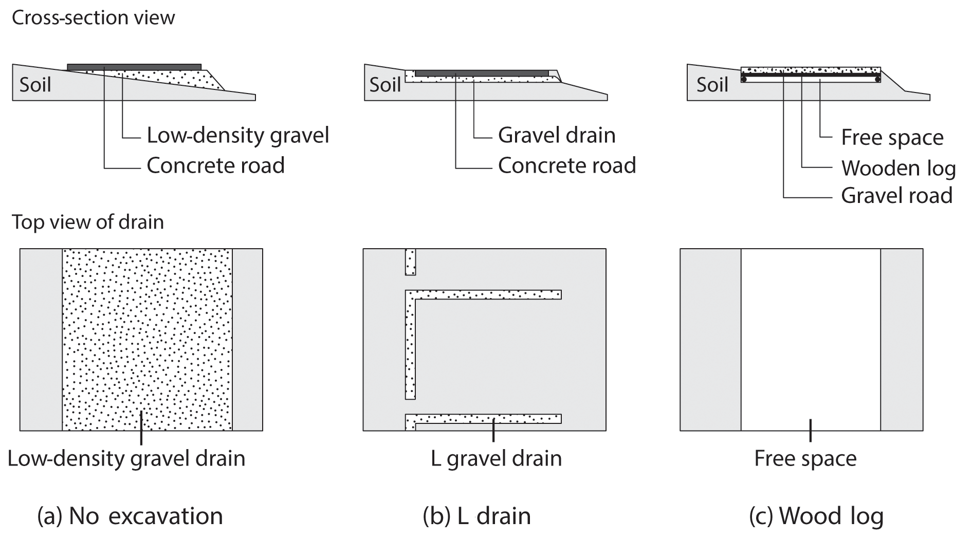
Figure 2Conceptual road structures: (a) no-excavation road structure, (b) L-drain road structure, and (c) wood-log road structure.
In Switzerland, more than 20 000 ha are included in the national inventory of fens of national importance (Broggi, 1990), and most of them are located in the mountainous regions of the northern Prealps. These fens developed on nearly impermeable geomorphological layers such as silty moraine material or a particular rock layer known as “flysch”. The majority of the remaining Swiss fens are sloping fens in this particular geological environment. To protect the remaining wetlands, it is important to reduce the impact of these constructions, be it in the context of replacing existing, old roads or for the construction of new roads.
The aim of this study is to investigate the hydrogeological impact of the three road structures and their effects on fen water dynamics to support decision-makers in choosing road structures with minimal impact. A combination of fieldwork and hydrogeological modeling tasks was employed. Fieldwork was used to document the hydrogeological impact of existing road structures on fen water dynamics. It is the first time that these road types have been systematically analyzed under field conditions. Sites with similar natural conditions were chosen to compare the influence of different road constructions on flow processes. The field studies allow for the assessment of the effectiveness of a given road structure at a particular location; however, they cannot provide a generalizable analysis of the different road types under different environmental and physical conditions. For example, critical environmental factors such as the slope or the bulk hydraulic properties of the fen will vary at different locations. This gap was filled by the development of generic numerical models. The most important hydraulic properties which control flow dynamics are explored systematically: the slopes of fens and the bulk hydraulic conductivity. The models are kept deliberately simple in terms of the heterogeneity of the soil. As the heterogeneity of the soil is not considered in the models, the horizontal redistribution due to field-specific heterogeneity cannot be considered (see Fig. 1c). Thus, the simulations constitute a “worst-case” scenario, which allows for a systematic comparison and a relative ranking of the different road structures in terms of perturbation and the risk of gully erosion.
2.1 Study areas and fieldwork
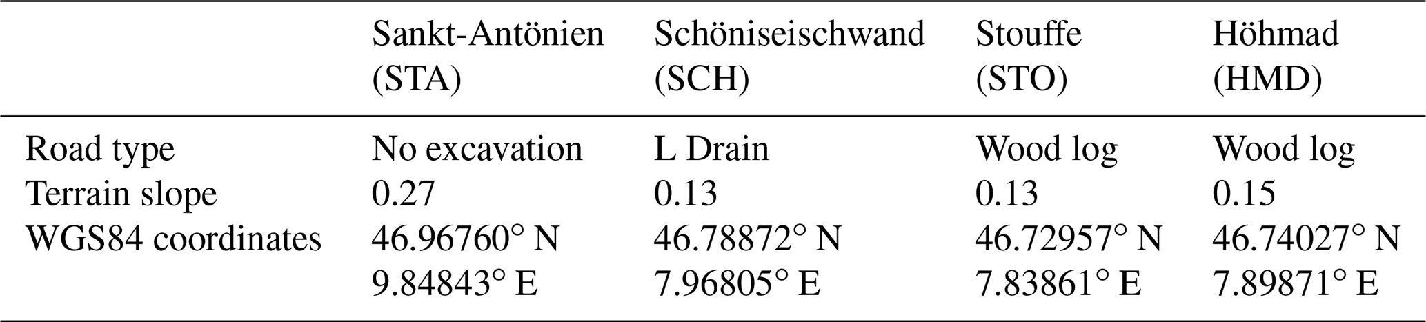
Four sloping fen areas located in alpine or peri-alpine regions of Switzerland (Table 1) were identified for this study. All areas are situated in protected fen areas, and their selection was based on two main criteria:
-
the subsurface water flow must occur only in the topsoil layer and as runoff (as described in the introduction), and
-
roads constructed with either a no-excavation, an L-drain, or a wood-log structure must be present.
To fulfill the first criteria, soil profiles were analyzed to ensure that each area with different road types had the comparable soil stratigraphy: it had to be composed of organic soil on top of a layer of impermeable clay and similar hydraulic regimes (e.g., runoff and subsurface flow occurring only in the topsoil layer). In addition, to ensure that subsurface water is forced to cross the road instead of flowing parallel to the road (and thus not being directly affected by the road), another important criterion for the selection of the study areas was that the subsurface flow was perpendicular to the road.
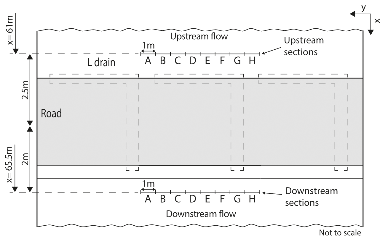
To evaluate the hydraulic connection provided by the roadbed structures, tracer tests were carried out. As illustrated schematically in Fig. 3, the upslope area was irrigated with a saline solution and the occurrence of the tracer was monitored downslope of the road. In the absence of surface runoff, the occurrence of a tracer downslope demonstrates the hydrogeological connection through the road. Furthermore, the spatial distribution of the tracer front reflects the heterogeneity of the flow paths.
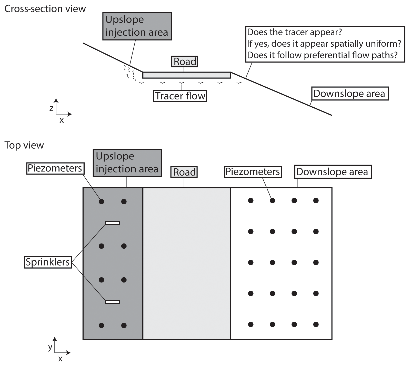
At each field site, an area of an 8 m × 20 m rectangle that included a 2.5 to 3.5 m wide road segment was selected. A network of approximately 30 mini-piezometers was installed on both sides of the road (Fig. 3) to monitor the hydraulic heads and was used to obtain samples for the tracer test.
The mini-piezometers are high-density polyethylene (HDPE) tubes no longer than 1.5 m (i.d. of 24 mm). Each tube was screened with 0.4 mm slots from the bottom end to 5 cm below ground level. They were inserted into the soil after extracting a core with a manual auger (diameter of 4–6 cm). The gap between the tube and the soil was filled with fine gravel and sealed on the top with a 4 cm thick layer of bentonite or local clay. Hydraulic heads were measured using a manual water level meter (±0.3 cm). At each point, the terrain and the top of the piezometer were leveled using a level (±0.3 cm), whereas the horizontal position was measured with a tape measure (±5 cm).
The tracer tests were conducted using two oscillating sprinklers designed to reproduce a 30 mm rain event over 2–3 h. This is equivalent to an intense rain event. Prior to the experiment, the sprinklers were activated for 15–60 min to wet the soil surface. Sodium chloride was added to the irrigated solution to obtain an electrical conductivity of 5–10 mS cm−1 which is approximately 10 times higher than the natural electrical conductivity of the groundwater. Subsequently, the area (60 m2) upslope of the road (upslope injection area of Fig. 3) was irrigated with the salt solution using the two sprinklers. The electrical conductivity (EC) of soil water was manually measured using a conductivity meter in all mini-piezometers prior to the experiment, immediately after the experiment, and 24 h after the experiment. An increase in EC in the piezometers located in the downslope area indicates that the injected saltwater flowed from the upslope area to the downslope area below the road and clearly shows a hydraulic connection. Conversely, if no changes in EC are observed in the piezometers, the hydraulic connection between the upslope and downslope of the road is affected.
2.2 Numerical modeling
The modeling approach was structured in three steps. First, a 3-D base case model representing surface and subsurface water flow in a sloping fen was elaborated. Subsequently, the base case model was modified to represent the three different types of road structures. For each model, various slopes, soil, and road drain hydraulic conductivities were implemented to produce a sensitivity analysis and explore their sensitivities in the sloping fen flow dynamics (see Sect. 2.2.3 for details).
2.2.1 Numerical simulator
The model used in the study is HydroGeoSphere (HGS; Aquanty, 2017). HGS is a physically based surface–subsurface fully integrated model, based on the blueprint of Freeze and Harlan (1969), who proposed a model structure for jointly simulating surface- and subsurface flow processes (Simmons et al., 2019). HGS uses the control volume finite element approach and solves a modified Richards' equation describing the 3-D subsurface flow. If the subsurface flow is unsaturated, HGS employs the van Genuchten (1980) functions to relate pressure head to saturation and relative hydraulic conductivity. Simultaneously, HGS solves the 2-D depth-averaged diffusion-wave approximation of the Saint-Venant equation for describing the surface flow. To couple surface and subsurface and simulate the water exchanges between both domains, the “dual node approach” is used. In this approach, the top nodes representing the ground surface are used for calculating both subsurface and surface flow, and the exchange flux between the two domains is calculated based on the head difference between the surface and the subsurface and a coupling factor.
The iterative Newton–Raphson method is used to solve the nonlinear equations. At each subsurface node, saturation and groundwater heads are calculated, which allows for the calculation of the Darcy flux. For further details on the code, HGS capabilities, and application, see Aquanty (2017), Brunner and Simmons (2012), or Cochand et al. (2019).
2.2.2 Conceptual models and model implementation
Figure 4 illustrates the conceptual model of each case. Existing engineering sketches were used as a basis for the implementation of the drain and road. Geometry, topography, and slopes are based on the conditions in the field. In each model, the soil layer has a thickness of 0.4 m and the surface and subsurface water originate from precipitation only. The upslope boundary is the catchment boundary (water divide) and the downslope boundary represents the outlet of the model. Finally, it is assumed that the layer beneath the soil is impermeable (as observed in the field). One Neumann (constant flux) boundary condition was used on the top face for simulating precipitation. A constant head (Dirichlet-type) boundary condition equal to the ground surface elevation (2 m) was used on the lowest cells of the slope (x=76 m in Fig. 5a) allowing groundwater to flow out of the model. Finally, a critical depth boundary condition which allows surface water to flow out of the model domain was implemented on the top nodes located at x=76 m. All other faces are no-flow boundary conditions.
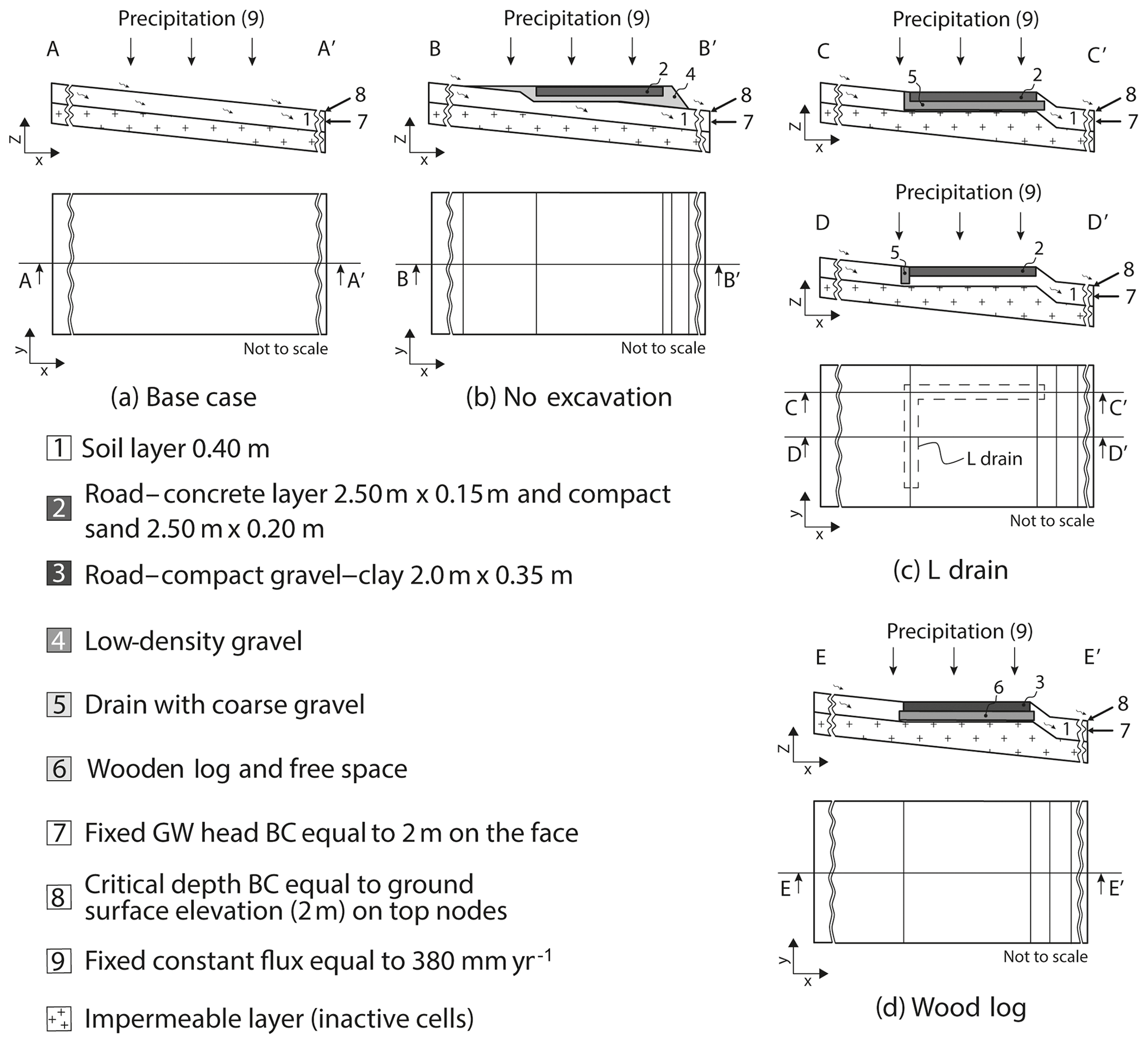
Figure 4(a) Base case, (b) no-excavation, (c) L-drain, and (d) wood-log structure conceptual models. BC refers to boundary conditions.
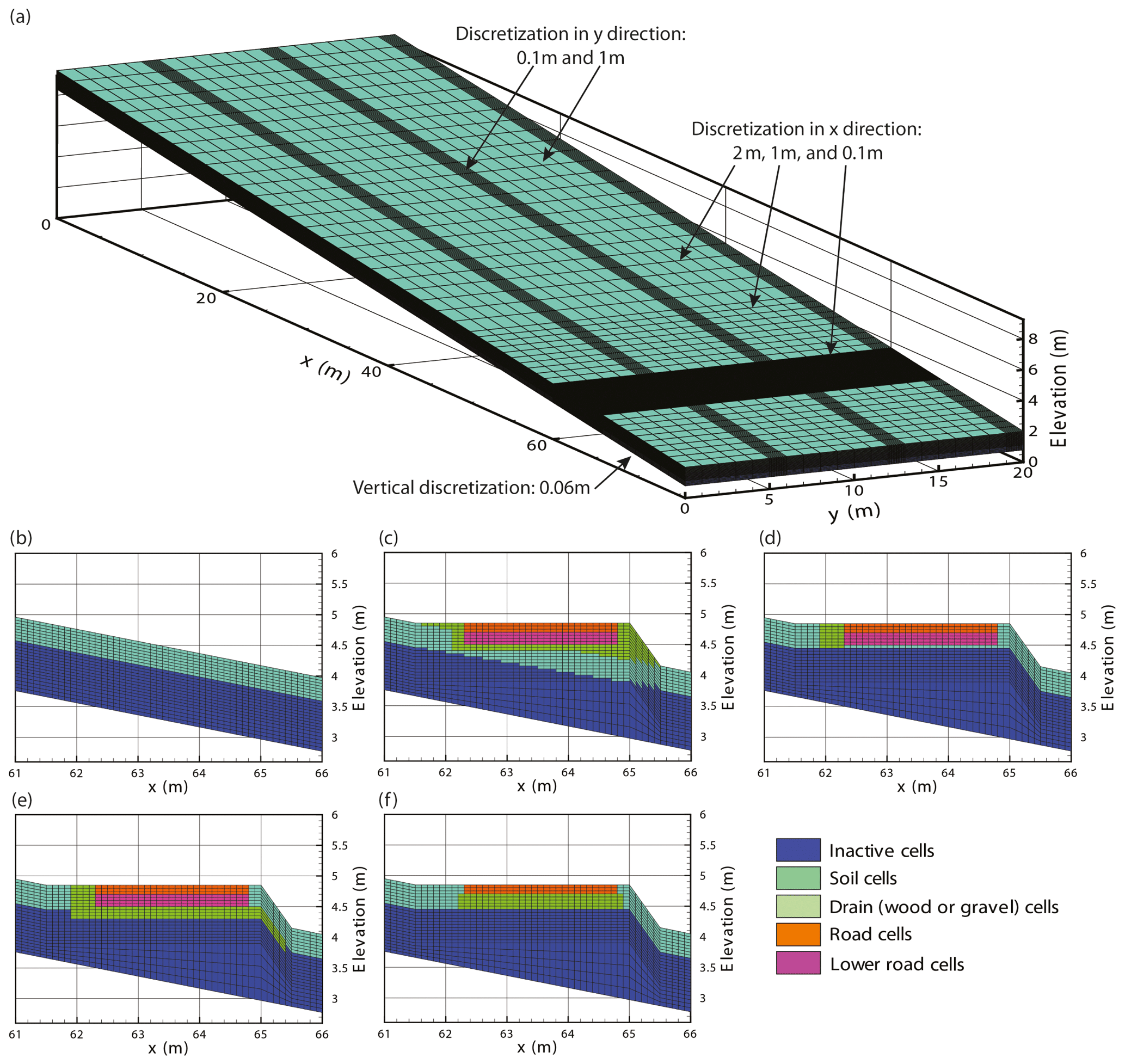
Figure 5Model development: (a) base case model, (b) base case model cross-section between 61 m <x and x<66 m, (c) no-excavation model between 61 m <x and x<66 m, (d) L-drain model between 61 m <x and x<66 m, (e) L-drain model between 61 m <x and x<66 m along the transversal drain, and (f) wood-log model between 61 m <x and x<66 m.
A 3-D finite element mesh was developed (Fig. 5a). The mesh was 76 m long in the x direction, 20 m in the y direction, and the mesh thickness was 1.2 m. The top elevation was fixed at 2 m on the right side (x=76 m) and varied from 9.6 to 24.8 m on the left side (x=0) according to the slope of the model. The mesh was composed of 24 layers, 127 200 nodes, and 118 440 rectangular prism elements. To guarantee numerical stability, mesh refinements were implemented. The element size varied between 2 and 0.1 m horizontally (in the x and y directions) and 0.09 and 0.06 m vertically.
The base case model and the three other models representing different road types have the same boundary conditions and finite element meshes; however, modifications were made between coordinates for the implementation of the different road types. Figure 5 depicts the differences between the base case model (Fig. 5a, b) and models with roads (Fig. 5c, d, e, f). In models simulating a road, the mesh and the material properties were adjusted. The fine spatial discretization of the mesh created between the coordinates allows a more accurate representation of the simulated processes where high hydraulic gradients are expected (near roads and drains).
2.2.3 Model application
The model application consists of the variation of model properties to assess their effect on the groundwater dynamics. The following parameters were analyzed: fen slope, soil hydraulic conductivities, and road drain hydraulic conductivities. These parameters were selected because according to Darcy's law (Eq. 1) they control the groundwater flow dynamics:
where K is the hydraulic conductivity of the soil and the drain, and ∇H is the hydraulic gradient of subsurface water in the fen, which itself strongly influenced by the topographical slope.
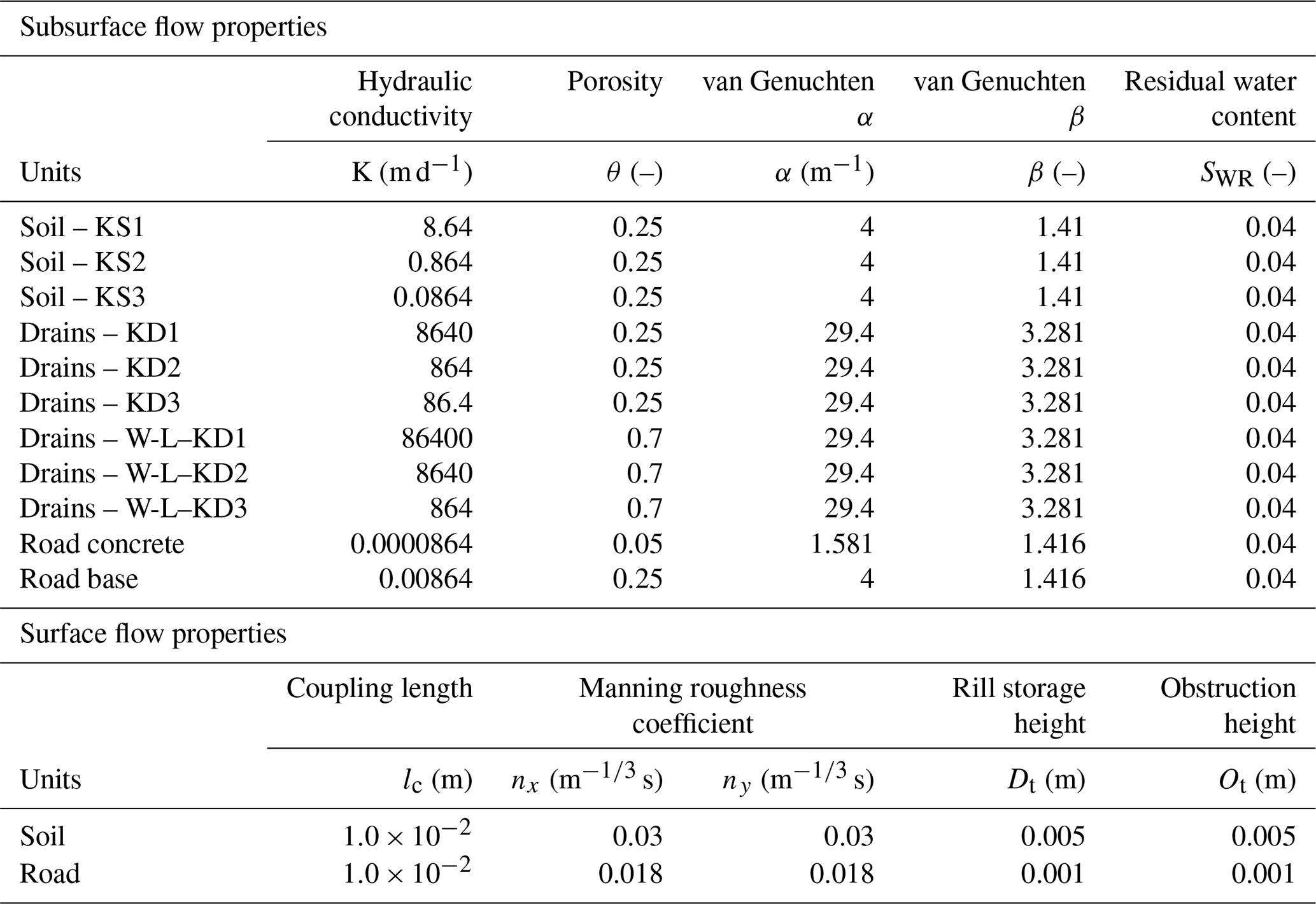
For each property varied in the sensitivity analysis, three different values were chosen (Table 2): a low, intermediate, and high value. For the soil hydraulic conductivities (KS), values presented in Chambers (2003) were used and varied between 8.64 and 0.0864 m d−1. This corresponds to a soil composed of gravely organic matter (as observed for example at the Sankt-Antönien site) or loamy organic matter (as observed for example at the Schöniseischwand site). The van Genuchten parameters (α and β), as well as the residual water content, were not varied. The road drains (KD) which are made of coarse or very coarse gravel were assigned a hydraulic conductivity between 8640 and 86.4 m d−1 (Fetter, 2001), with their van Genuchten parameters corresponding to gravel. The slopes were fixed at 10 %, 20 %, and 30 %, as observed during fieldwork. The hydraulic conductivities of the wood-log (W-L) drain were assumed to be 10 times more conductive and more porous than the gravel drain. The road concrete is almost impermeable; thus, it was conceptualized with a very low hydraulic conductivity, with its van Genuchten parameters corresponding to fine material. The road base is constructed using highly compacted fine material (sand and loam); thus, it was implemented with low hydraulic conductivity, with the van Genuchten parameters corresponding to fine material. Finally, the implemented soil and road surface flow properties correspond to a wetland and urban cover (Li et al., 2008).
In order to simulate each parameter combination, a total of 90 models were developed (27 models for each road structure and 9 models for natural conditions). Models were run for 10 000 d (about 27 years) with a constant flux equal to 380 mm yr−1 on the top, representing the rainfall to reach a steady state. Subsequently, subsurface flow rates in the soil layer were extracted at each section with an area of 0.4 m2 (1 m wide times the soil thickness) presented in Fig. 6. Changes in subsurface flow rates indicate a perturbation of flow dynamics; therefore, a comparison of flow rates between each model was made to present the effect of each road structure and sloping fen properties on the dynamics.
3.1 Fieldwork
Based on the observations, all sites show a continuous saturated zone before the experiment, both upslope and downslope of the road, with the hydraulic gradients being similar to the terrain slope (Fig. 7, first column). In contrast, the EC maps established prior to the tracer test show a spatial variability across one to several meters (Fig. 7, second column). Within each plot, EC varies from 482 to 629 µS cm−1. At the SCH site, the highest values are located downslope of the L-drain outlet which could indicate that the EC increases as water is flowing through the drain (e.g., through the dissolution of the construction material). Given that this initial distribution of EC is not uniform, the comparison of EC after the sprinkling experiment has to be made in a relative manner (Fig. 7, third column).
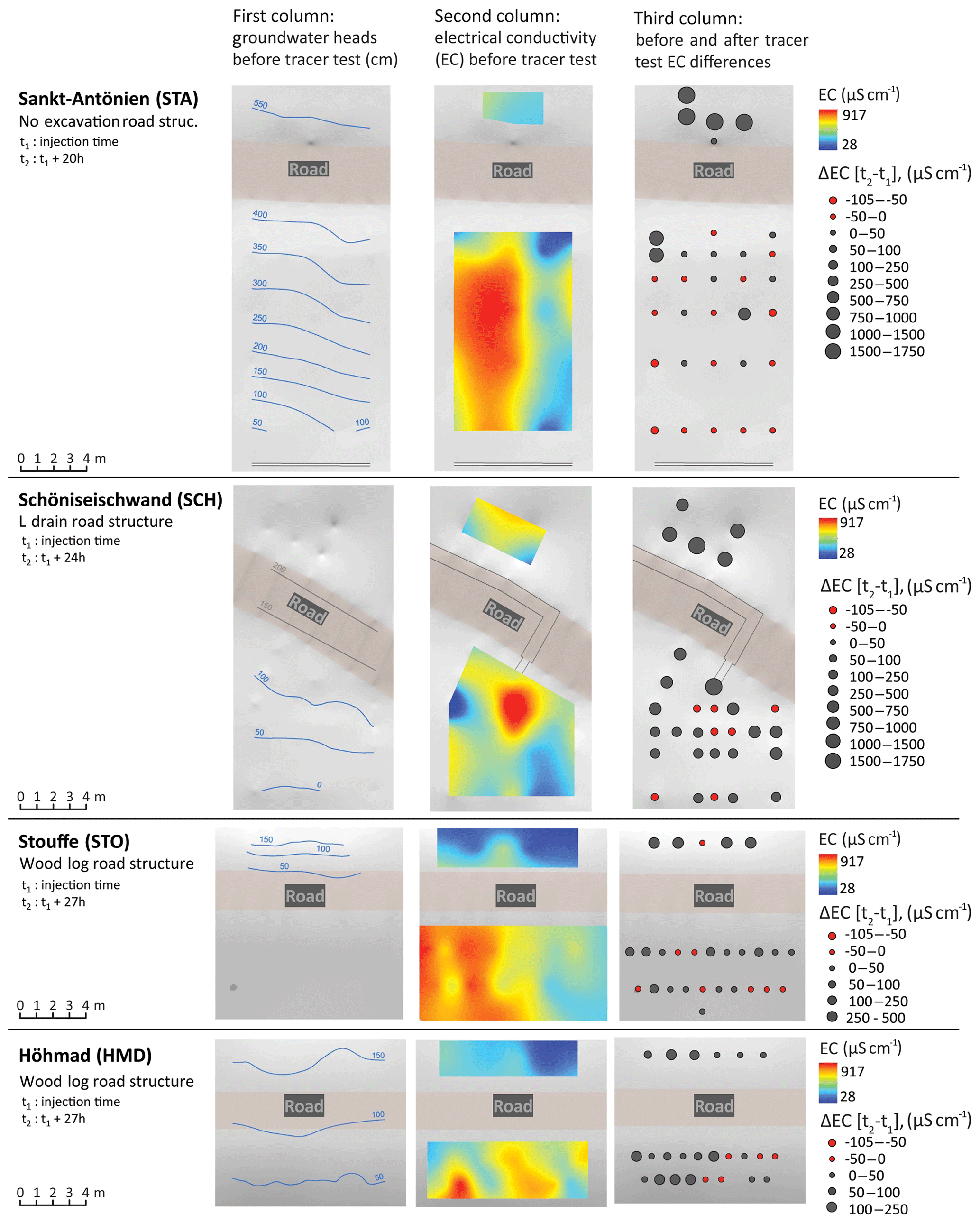
Figure 7Fieldwork results at the four field sites: the first column shows the measured groundwater heads before the tracer test, the second column shows the measured EC before the tracer test, and the third column shows the before and after tracer test differences in EC. The hydraulic head downslope of the road at the Stouffe site is about 25 cm, whereas that upslope of the road at the Schöniseischwand is about 225 cm (between two isolines); these values are not presented in the figure.
The heterogeneity of the hydraulic conductivity of the soil is apparent from the tracer tests (Fig. 7, third column: EC 24 h after injection). At all four sites, the front of the saline solution is not uniform due to the heterogeneity of the soil hydraulic conductivity. Nevertheless, the road structures or the drains may create preferential flow paths. This clearly occurs at the SCH site, where the front follows two preferential flow paths: one related to the L drain (right path) and the other unrelated to the L drain (left path). This suggests that the latter drains only a part of the water and that the remaining water follows a natural preferential flow path. At the HMD site, the saline solution is far more concentrated on the left side of the plot; however, this is apparently not as a result of the road's structure. Rather, the soil appears more permeable on the left side of the plot, both upslope and downslope of the road. Finally, the decrease in EC observed 24 h after injection at some locations might result from the following: (1) the tracer injection induces the displacement of a small volume of local water with a lower EC, via “piston effect”; (2) the tracer injection was preceded by a period of irrigation without tracer. This could have diluted the pre-irrigation soil solution.
In each case, the irrigation experiments demonstrate the continuity of subsurface flow under the road for all structures. For the no-excavation and wood-log type, the perturbation of the flow field seems to be controlled by the natural heterogeneity of the soil and flow paths, and not by the road itself. Conversely, the field data suggest that the L drain constitutes a preferential pathway. This flow convergence can cause gully erosion.
3.2 Modeling
Figure 8a shows the results of the models with a slope of 10 %, Fig. 8b shows the results for a slope of 20 %, and Fig. 8c shows the results for a slope of 30 %. In each panel, the groundwater flow rates (always in cubic meters per day, m3 d−1) are plotted using crosses for the base case model, diamonds for the no-excavation model, squares for the L-drain model, and circles for the wood-log model. In addition, the maximum flow rate capacity of the soil calculated with Darcy's Law (Eq. 1) and the flow rate induced by precipitation are also presented for the interpretation of the results. In the following paragraphs, the base case (natural conditions) results are presented and discussed, followed by the simulations of the road structures.
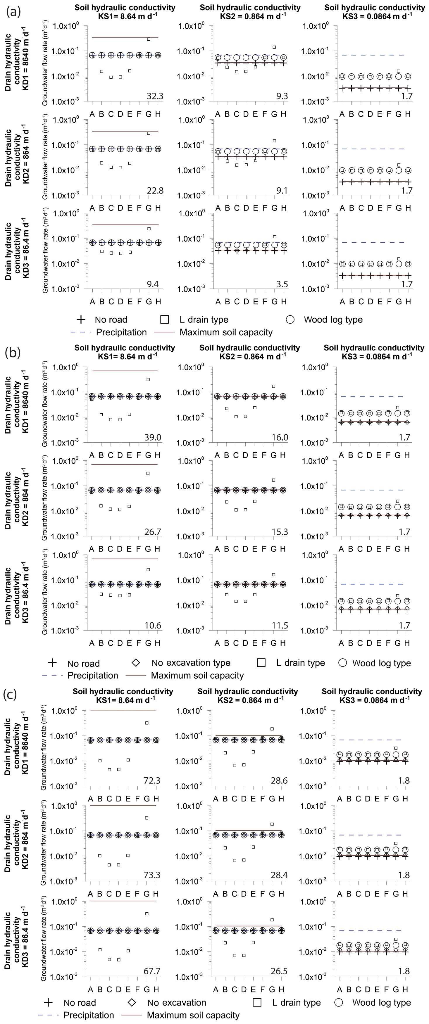
Figure 8Simulated groundwater flow rates 2 m downslope of each road structure and each parameter combination with a slope of (a) 10 %, (b) 20 %, and (c) 30 %. Numbers in the bottom right corner of each panel represent the ratio between the maximum and minimum groundwater flow within the L-drain transect.
In the base case model, groundwater flow rates vary from 0.003 to 0.069 m3 d−1 for a 10 % slope, from 0.006 to 0.069 m3 d−1 for a 20 % slope, and from 0.009 to 0.069 m3 d−1 for a 30 % slope. The groundwater flow rate decreases following a decrease in the hydraulic conductivities (KS) of the soil layer. The groundwater flow rates are mainly controlled by the hydraulic conductivities, and the slope plays a less important role. This is expected, as the ratios of the maximum and minimum hydraulic conductivity span 2 orders of magnitude, while slopes were multiplied by a factor of 2 (for a slope of 20 %) or 3 (for a slope of 30 %). Therefore, groundwater flow is increased by a factor 3 between the model KS3 with a slope of 10 % and model KS3 with a slope of 30 %. Concerning the formation of surface flow, the following observation can be made: for all KS2 and KS3 models, surface flow occurs, while the infiltration capacity of the KS1 models is never exceeded and, thus, no surface flow occurs.
In the no-excavation and wood-log models, the influence on flow rates caused by the presence of the road structures is quite similar. Groundwater flows vary from 0.01 to 0.069 m3 d−1 for a 10 % slope, from 0.01 to 0.069 m3 d−1 for a 20 % slope, and from 0.010 to 0.069 m3 d−1 for a 30 % slope. Compared with the base case model, results show that the no-excavation and wood-log structures have a minimal impact on flow perturbation. The only marked difference is that groundwater flow rates are slightly higher if the soil hydraulic conductivities are low (KS3). This is due to the hydraulic conductivity of the base of the road (consisting of wood logs) being higher than the hydraulic conductivity of the soil which facilitates infiltration. Conversely, in the base case model, less water infiltrates and more surface runoff occurs. In the 20 % and 30 % slope models, the results of the no-excavation model are similar to the base case model.
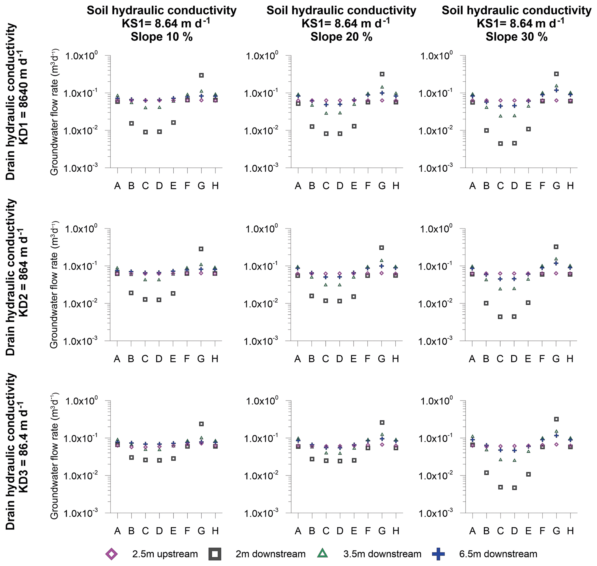
Figure 9Extent of perturbations due to the L-drain road type: simulated groundwater flow rates at different distances from the road.
In the L-drain model, the effect of the road is markedly different from the other road structures. The groundwater flows vary significantly with respect to the observation sections. The maximum flows are always obtained in observation section G (see Fig. 6 for the location of the sections) just downslope of the drain outlet and can be 10 times higher than the base case. Conversely, minimum flows are obtained in observation sections C and D in which flow rates can be 10 times lower. Significant differences in groundwater flow are also observed in the same transect (within the same model). To condense this information, the ratios between maximum and minimum flow rates are calculated for the L-drain structures (numbers in the bottom right corners of the panels in Fig. 8). The maximum differences are observed for the cases where the hydraulic conductivity of the soil (KS) and drain (KD) are high and vary from 0.025 to 0.150 m3 d−1. Conversely, when KS and/or KD is low, the differences along the transect are smaller. Finally, the slope accentuates the groundwater flow rate differences along the transect. Therefore, an increase in the groundwater flow differences is observed for the 10 % and 30 % slope scenarios, within the same model. The impact of the L drain may be further explored by extracting groundwater flows lower than 2 m downslope of the road to assess the extent of perturbations. Figure 9 shows simulated groundwater flows for the most critical cases (i.e., KS1 with a slope of 10 %, 20 %, and 30 %) downslope of the road at 3.5 and 6.5 m, respectively, and 2.5 m upslope. At 3.5 m downslope, groundwater flow regains the upslope conditions. At 6.5 m downslope of the road, all observation sections are very similar to the upslope flows except in section G where flows are still slightly higher.
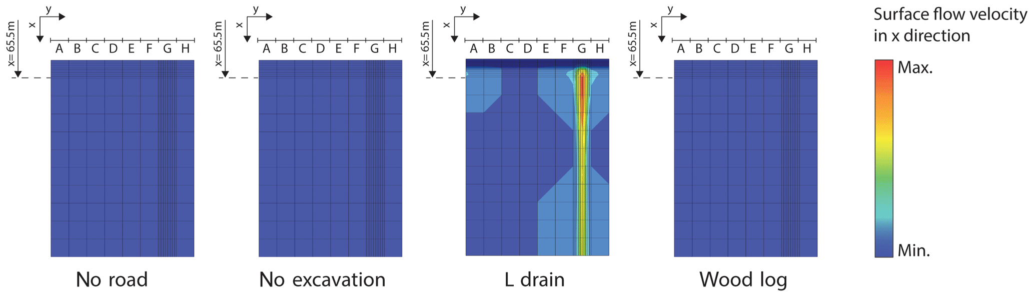
Figure 10Simulated surface flow of the KS2–KD2 model and a slope of 20 % for each road structure (min. velocity =0 m d−1 and max. velocity =0.25 m d−1). The results clearly indicate the increased risk caused by the L drain with respect to triggering surface runoff and, in turn, potential gully erosion and sections of the wetland drying out.
In addition to the assessment of perturbation due to roads, the model results can be used to evaluate the risk of gully erosion. As presented in Fig. 8, the maximum flow rate capacity of the soil is small in comparison to precipitation. For all model scenarios except for KS1, the soil capacity is lower than the precipitation and, thus, surface runoff occurs in the models and is likely to occur naturally. However, surface runoff may be triggered by the presence of L-drain structures. To illustrate this process, the simulated surface flow velocities of each road structure downslope of the road for the model KS2–KD2 and a slope of 20 % are presented in Fig. 10. In this case, the maximum flow rate capacity of the soil is approximately equal to precipitation, and therefore runoff should not occur. However, this is not the case for the L drain. The occurrence of surface runoff is a consequence of the subsurface flow concentration. In this configuration, the infiltration capacity of the soil is too small to accommodate the concentrated flow collected upslope, thus groundwater emerges and surface flow is triggered. This constitutes an increased risk of gully erosion. In addition, the perturbation of roads upslope of the road was assessed.
Finally, the impact of road structure on the upslope road dynamics was also assessed (figure not shown) 2.5 m upslope. Upslope flows are similar to the base case model; thus, the influence of the road is, not unexpectedly, marginal for all road types.
The development of models with various combinations of parameters allowed for the exploration of a larger parameter space than fieldwork alone. For instance, the fact that the impact of an L-drain structure on the water dynamics is less marked if the hydraulic conductivity of soil is low would have been impossible to identify using just fieldwork. However, a numerical model is always a simplified reproduction of reality. The main model assumption is that the hydraulic conductivity of the soil is homogeneous – as opposed to the field conditions analyzed. However, the models are not intended to reproduce small-scale observations, i.e., the exact hydraulic head in a piezometer, but instead can be used to explore the influence of the road structures under different soil conditions (bulk hydraulic conductivities and slopes). Given that no heterogeneity-induced horizontal redistribution of the flow downslope can be simulated using homogeneous soil conditions, the models constitute a worst-case scenario. It is a worst-case scenario because we exclude the possibility that a fraction of the drained water could be horizontally redistributed downstream through natural heterogeneity, thereby potentially reducing the negative impact of the road. Therefore, the models allow for a relative ranking of the potential impact and clearly show the increased risk of surface water flow generation and, in turn, gully erosion. For the scenarios investigated, the L drain consistently shows the largest impact. Thus, the other two road structures are the preferred construction types.
This study assessed three road structures with respect to their perturbations of the natural groundwater flow. Two of these road structures were specifically developed to reduce the negative impacts of the road. The study is based on two complementary approaches: field-based tracer tests and numerical models simulating groundwater flow for the different road structures. The combination of fieldwork and the development of numerical models was fundamental to achieving the goal of this study. The tracer test allowed for a better understanding of groundwater flow through road structures and allowed for an evaluation of their effectiveness at a given location. However, the tracer tests are time-consuming and only a few suitable field sites are available. Moreover, the results are site-specific. The numerical approach, in contrast, allows for the exploration of any combination of slope, hydraulic properties, and road structure, thereby providing a more comprehensive approach aimed at a relative ranking of the influence of the road structure. Given the simplified structure of the models, the results can not be directly used to predict the influence at a specific field site.
For all scenarios investigated, the significant impact of the L-drain road structure is clearly established and is consistent with the field observations. For the other road structures, the numerical models are also consistent with fieldwork results and show a relatively undisturbed groundwater flow downslope of the road.
It is the first time that the performance of these road structures has been investigated in the field. The tracer tests showed that both sides of the road were hydraulically connected for all of the road structures investigated. Groundwater flow was heterogeneous suggesting the occurrence of natural preferential flow paths in the soil. The presence of a transversal drain (L drain) beneath the road suggests that the L drain constitutes a preferential flow path of much greater importance than the naturally occurring preferential pathways. The field results further suggest that the wood-log and no-excavation structures are less impactful than the L drain. The simulation results are consistent with the assessment of the relative impact of the different road types. Groundwater flow rates 10 times higher than the natural case were obtained in the numerical simulations. The two other road structures (wood log and no excavation) did not perturb the flow field to the extent of the L drain. To minimize the perturbation of flow fields, the wood-log and no-excavation structures are recommended.
Permission is required to use the data presented in this study; the corresponding author can assist those seeking access to the data.
FC, DH, and PB designed the study and wrote the paper. PG initiated the study and contributed to the design and execution of the experiments. Finally, DK carried out fieldwork and wrote parts of the paper.
The authors declare that they have no conflict of interest.
The authors are grateful to Léa Tallon, Benoit Magnin, Peter Staubli, Andreas Stalder, Anton Stübi, and Ueli Salvisberger for their collaboration. We thank the three anonymous reviewers as well as the editor, Anke Hildebrandt, for the very detailed input on the paper.
This research has been supported by the Swiss Federal Office for the Environment (FOEN) and the Swiss Federal Office for Agriculture (FOAG).
This paper was edited by Anke Hildebrandt and reviewed by Alraune Zech and two anonymous referees.
Aquanty: HydroGeoSphere: A Three-Dimensional Numerical Model Describing Fully-Integrated Subsurface and Surface Flow and Solute Transport, University of Waterloo, Waterloo, ON, Canada, 2017.
Baker, C., Thompson, J. R., and Simpson, M.: 6. Hydrological Dynamics I: Surface Waters, Flood and Sediment Dynamics The Wetlands Handbook, 1st edn., edited by: Maltby, E. and Barker, T., Blackwell Publishing, Chichester, UK, 120–168, 2009.
Betts, H. D. and DeRose, R. C.: Digital elevation models as a tool for monitoring and measuring gully erosion, Int. J. Appl. Earth Obs., 1, 91–101, https://doi.org/10.1016/S0303-2434(99)85002-8, 1999.
Broggi, M. E.: Minimum requis de surfaces proches de l'état naturel dans le paysage rural, illustré par l'exemple du Plateau suisse, Rapport 31a du Programme national de recherche “Sol”, Liebefeld-Berne, Switzerland, 199 pp., 1990.
Brunner, P. and Simmons, C. T.: HydroGeoSphere: a fully integrated, physically based hydrological model, Groundwater, 50, 170–176, 2012.
Capra, A., Porto, P., and Scicolone, B.: Relationships between rainfall characteristics and ephemeral gully erosion in a cultivated catchment in Sicily (Italy), Soil Till. Res., 105, 77–87, https://doi.org/10.1016/j.still.2009.05.009, 2009.
Chambers, F.: Peatlands and environmental change, edited by: Charman, D., John Wiley and Sons Ltd, Chichester, UK, 2002, 301 pp., ISBN 0471969907 (HB) 0471844108 (PB), J. Quaternary Sci., 18, 466–466, https://doi.org/10.1002/jqs.741, 2003.
Chimner, R. A., Cooper, D. J., Wurster, F. C., and Rochefort, L.: An overview of peatland restoration in North America: where are we after 25 years?, Restor. Ecol., 25, 283–292, 2016.
Cochand, F., Therrien, R., and Lemieux, J.-M.: Integrated Hydrological Modeling of Climate Change Impacts in a Snow-Influenced Catchment, Groundwater, 57, 3–20, https://doi.org/10.1111/gwat.12848, 2019.
Cognard Plancq, A. L., Bogner, C., Marc, V., Lavabre, J., Martin, C., and Didon Lescot, J. F.: Etude du rôle hydrologique d'une tourbière de montagne: modélisation comparée de couples “averse-crue” sur deux bassins versants du Mont-Lozère, Etudes de géographie physique, no. XXXI, 3–15, 2004.
Daba, S., Rieger, W., and Strauss, P.: Assessment of gully erosion in eastern Ethiopia using photogrammetric techniques, Catena, 50, 273–291, https://doi.org/10.1016/S0341-8162(02)00135-2, 2003.
Derose, R. C., Gomez, B., Marden, M., and Trustrum, N. A.: Gully erosion in Mangatu Forest, New Zealand, estimated from digital elevation models, Earth Surf. Proc. Land., 23, 1045–1053, https://doi.org/10.1002/(SICI)1096-9837(1998110)23:11<1045::AID-ESP920>3.0.CO;2-T, 1998.
Descroix, L., González Barrios, J. L., Viramontes, D., Poulenard, J., Anaya, E., Esteves, M., and Estrada, J.: Gully and sheet erosion on subtropical mountain slopes: Their respective roles and the scale effect, Catena, 72, 325–339, https://doi.org/10.1016/j.catena.2007.07.003, 2008.
Dutton, A. L., Loague, K., and Wemple, B. C.: Simulated effect of a forest road on near-surface hydrologic response and slope stability, Earth Surf. Proc. Land., 30, 325–338, https://doi.org/10.1002/esp.1144, 2005.
Fetter, C. W.: Applied Hydrogeology, 4th edn., Prentice-Hall, New Jersey, USA, 2001.
Freeze, R. A. and Harlan, R. L.: Blueprint for a physically-based, digitally-simulated hydrologic response model, J. Hydrol., 9, 237–258, https://doi.org/10.1016/0022-1694(69)90020-1, 1969.
Li, Q., Unger, A. J. A., Sudicky, E. A., Kassenaar, D., Wexler, E. J., and Shikaze, S.: Simulating the multi-seasonal response of a large-scale watershed with a 3D physically-based hydrologic model, J. Hydrol., 357, 317–336, https://doi.org/10.1016/j.jhydrol.2008.05.024, 2008.
Limpens, J., Berendse, F., Blodau, C., Canadell, J. G., Freeman, C., Holden, J., Roulet, N., Rydin, H., and Schaepman-Strub, G.: Peatlands and the carbon cycle: from local processes to global implications – a synthesis, Biogeosciences, 5, 1475–1491, https://doi.org/10.5194/bg-5-1475-2008, 2008.
Lindsay, R.: Peatbogs and carbon: a critical synthesis to inform policy development in oceanic peat bog conservation and restoration in the context of climate change, University of East London, Technical Report, London, UK, 2010.
Loague, K. and VanderKwaak, J. E.: Simulating hydrological response for the R-5 catchment: comparison of two models and the impact of the roads, Hydrol. Process., 16, 1015–1032, https://doi.org/10.1002/hyp.316, 2002.
Martínez-Casasnovas, J. A.: A spatial information technology approach for the mapping and quantification of gully erosion, Catena, 50, 293–308, https://doi.org/10.1016/S0341-8162(02)00134-0, 2003.
Nyssen, J., Poesen, J., Moeyersons, J., Luyten, E., Veyret-Picot, M., Deckers, J., Haile, M., and Govers, G.: Impact of road building on gully erosion risk: a case study from the Northern Ethiopian Highlands, Earth Surf. Proc. Land., 27, 1267–1283, https://doi.org/10.1002/esp.404, 2002.
Partington, D., Therrien, R., Simmons, C. T., and Brunner, P.: Blueprint for a coupled model of sedimentology, hydrology, and hydrogeology in streambeds, Rev. Geophys., 55, 287–309, https://doi.org/10.1002/2016rg000530, 2017.
Poesen, J., Nachtergaele, J., Verstraeten, G., and Valentin, C.: Gully erosion and environmental change: importance and research needs, Catena, 50, 91–133, https://doi.org/10.1016/S0341-8162(02)00143-1, 2003.
Reckendorfer, W., Funk, A., Gschöpf, C., Hein, T., and Schiemer, F.: Aquatic ecosystem functions of an isolated floodplain and their implications for flood retention and management, J. Appl. Ecol., 50, 119–128, 2013.
Reid, L. M. and Dunne, T.: Sediment production from forest road surfaces, Water Resour. Res., 20, 1753–1761, https://doi.org/10.1029/WR020i011p01753, 1984.
Rydin, H. and Jeglum, J. K.: The biology of peatlands, 2nd edn., Oxford University Press, Oxford, UK, 382 pp., 2005.
Samaritani, E., Siegenthaler, A., Yli-Petäys, M., Buttler, A., Christin, P.-A., and Mitchell, E. A. D.: Seasonal Net Ecosystem Carbon Exchange of a Regenerating Cutaway Bog: How Long Does it Take to Restore the C-Sequestration Function?, Restor. Ecol., 19, 480–489, https://doi.org/10.1111/j.1526-100X.2010.00662.x, 2011.
Simmons, C. T., Brunner, P., Therrien, R., and Sudicky, E. A.: Commemorating the 50th anniversary of the Freeze and Harlan (1969) Blueprint for a physically-based, digitally-simulated hydrologic response model, J. Hydrol., 124309, https://doi.org/10.1016/J.JHYDROL.2019.124309, in press, 2019.
Valentin, C., Poesen, J., and Li, Y.: Gully erosion: Impacts, factors and control, Catena, 63, 132–153, https://doi.org/10.1016/j.catena.2005.06.001, 2005.
VanderKwaak, J. E.: Numerical simulation of flow and chemical transport in integrated surface-subsurface hydrologic systems, PhD thesis, Departement of Earth Science, University of Waterloo, Waterloo, Ontario, Canada, 1999.
Van Genuchten, M. T.: A closed-form equation for predicting the hydraulic conductivity of unsaturated soils, Soil Sci. Soc. Am. J., 44, 892–898, 1980.
Von Sengbusch, P.: Enhanced sensitivity of a mountain bog to climate change as a delayed effect of road construction, Mires and Peat, 15, 6, available at: http://www.mires-and-peat.net/pages/volumes/map15/map1506.php (last access: 23 February 2018), 2015.
Wemple, B. C. and Jones, J. A.: Runoff production on forest roads in a steep, mountain catchment, Water Resour. Res., 39, 1220, https://doi.org/10.1029/2002wr001744, 2003.
Zollner, A.: Das Abflussgeschehen von unterschiedlich genutzten Hochmooreinzugsgebieten, Bayer. Akad. f. Naturschutz u. Landschaftspflege, Laufener Seminarbeitr., Laufen/Salzach, Germany, 111–119, 2003.