the Creative Commons Attribution 4.0 License.
the Creative Commons Attribution 4.0 License.
 | 11 May 2020
A line-integral-based method to partition climate and catchment effects on runoff
It is a common task to partition the synergistic impacts of drivers in the environmental sciences. However, there is no mathematically precise solution to this partition task. Here I present a line-integral-based method, which addresses the sensitivity to the drivers throughout the drivers' evolutionary paths so as to ensure a precise partition. The method reveals that the partition depends on both the change magnitude and pathway (timing of the change) but not on the magnitude alone unless used for a linear system. To illustrate this method, I applied the Budyko framework to partition the effects of climatic and catchment conditions on the temporal change in the runoff for 19 catchments from Australia and China. The proposed method reduces to the decomposition method when assuming a path in which climate change occurs first, followed by an abrupt change in catchment properties. The proposed method re-defines the widely used sensitivity at a point as the path-averaged sensitivity. The total-differential and the complementary methods simply concern the sensitivity at the initial and/or the terminal state, so they cannot give precise results. Although the path-averaged sensitivities varied greatly among the catchments, they can be readily predicted within the Budyko framework. As a mathematically accurate solution, the proposed method provides a generic tool for conducting quantitative attribution analyses.
- Article
(1212 KB) -
Supplement
(320 KB) - BibTeX
- EndNote


The impacts of certain drivers on observed changes of interest often require quantification in environmental sciences. In the hydrology community, both climate and human activities have posed global-scale impact on hydrologic cycle and water resources (Barnett et al., 2008; Xu et al., 2014; Wang and Hejazi, 2011). Diagnosing their relative contributions to runoff is of considerable relevance to the researchers and managers. Unfortunately, performing a quantitative attribution analysis of runoff changes remains a challenge (Wang and Hejazi, 2011; Berghuijs and Woods, 2016; Zhang et al., 2016); this is to a considerable degree due to a lack of a mathematically precise method of decoupling synergistic and often confounding impacts of climate change and human activities.
Numerous studies have detected the long-term variability in runoff and attempted to partition the effects of climate change and human activities through various methods (Dey and Mishra, 2017); these include the paired-catchments method and the hydrological modeling method. The paired-catchment method can filter the effect of climatic variability and thus isolate the runoff change induced by vegetation changes (Brown et al., 2005). However, this method is capital intensive; moreover, it generally involves small catchments and experiences difficulties when extrapolating to large catchments (Zhang et al., 2011). Physically based hydrological models often have limitations such as a high data requirement, labor-intensive calibration and validation processes, and inherent uncertainty and interdependence in parameter estimations (Binley et al., 1991; Wang et al., 2013; Liang et al., 2015). Conceptual models such as Budyko-type equations (see Sect. 2.1) have consequently gained interest in recent years.
Within the Budyko framework, studies (Roderick and Farquhar, 2011; Zhang et al., 2016) have used the total differential of runoff as a proxy for the runoff change and the partial derivatives as the sensitivities (hereafter called the total-differential method). The total differential, however, is simply a first-order approximation of the observed change (Fig. 1a). This approximation has caused an error in the calculation of climate impact on runoff, with the deviation ranging from 0 to m (or −118 to 174 %) in China (Yang et al., 2014). The elasticity method proposed by Schaake (1990) is also based on the total-differential expression (Sankarasubramanian et al., 2001; Zheng et al., 2009). The method uses the “elasticity” concept to assess the climate sensitivity of runoff. The elasticity coefficients, however, have been estimated in an empirical way and are not physically sound (Roderick and Farquhar, 2011; Liang et al., 2015).
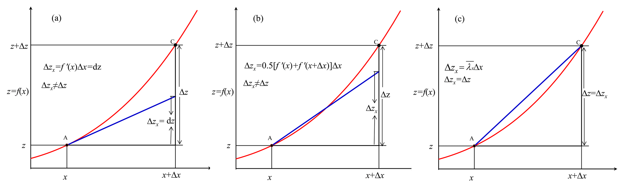
Figure 1For a nonlinear function z=f(x), the total-differential method (a) and the complementary method (b) do not accurately estimate the effect (Δzx) of x on z when x changes by Δx, but the LI method (c) does. For a univariate function, the z change is exclusively driven by x, so that Δzx should be equal to Δz. Δzx=Δz in (c) but not in (a) and (b). in (c) represents the average sensitivity along the curve AC and ; see Appendix E for details.
The so-called decomposition method developed by Wang and Hejazi (2011) has also been widely used. The method assumes that climate changes cause a shift along a Budyko curve and then human interferences cause a vertical shift from one Budyko curve to another (Fig. 2). Under this assumption, the method extrapolates the Budyko models that are calibrated using observations of the reference period, in which human impacts remain minimal, to determine the human-induced runoff changes that occur during the evaluation period.
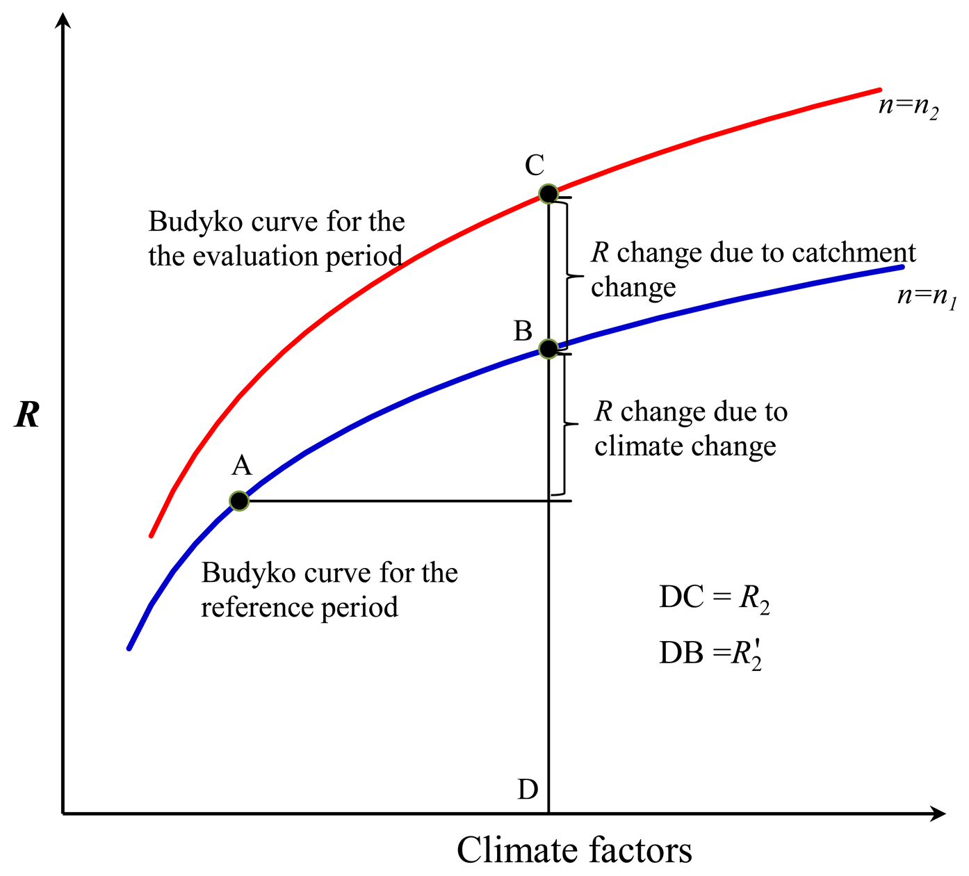
Figure 2A schematic plot illustrating the decomposition method. Point A denotes the initial state (the reference period), and point C denotes the terminal state (the evaluation period). The decomposition method assumes that the catchment state first evolves from Point A to B along the Budyko curve for the reference period, then jumps to Point C. R2 represents the mean annual runoff of the evaluation period, and R2′ the mean annual runoff given the climate conditions of the evaluation period and the catchment conditions of the reference period. See Sect. 2.4 for details.
Recently, Zhou et al. (2016) established a Budyko complementary relationship for runoff and further applied it to partitioning the climate and catchment effects. Superior to the total-differential method, the complementary method culminates by yielding a no-residual partition. Nevertheless, this method depends on a given weighted factor that is determined in an empirical but not a precise way. Furthermore, Zhou et al. (2016) argued that the partition is not unique in the Budyko framework because the path of the climate and catchment changes cannot be uniquely identified.
Obtaining a precise partition remains difficult, even when giving a precise mathematical model. This difficulty can be illustrated by using a precise hydrology model R=f (x, y), where R represents runoff, and x and y represent the climate factors and catchment characteristics, respectively. We assumed that R changes by ΔR when x changes by Δx and y changes by Δy; i.e., . To determine the effect of x on ΔR – i.e., ΔRx – a common practice is to assume that y remains constant when x changes by Δx. We thus obtain . Similarly, we can obtain . Although this derivation seems quite reasonable, it is problematic as . A further examination shows that a variable's effect on R seems to differ depending on the changing path (timing of the change). For example, and if x changes first and y subsequently changes (note that the partition is precise with at this moment). If y changes first and x subsequently changes, the partition then becomes and . In the case of x and y changing simultaneously, unfortunately, the current literature seems not to provide a mathematically precise solution.
The aim of this study is to propose a mathematically precise method to conduct a quantitative attribution to drivers. The method is based on the line integer (called the LI method hereafter) and takes into account the sensitivity throughout the evolutionary path of the drivers rather than at a point as the total-differential method does. To present and evaluate the proposed method, I decomposed the relative influences of climate and catchment conditions on runoff within the Budyko framework using data from 19 catchments from Australia and China.
2.1 Budyko framework and the MCY equation
Budyko (1974) argued that mean annual evapotranspiration (E) is largely determined by the water and energy balance of a catchment. Using precipitation (P) and potential evapotranspiration (E0) as proxies for water and energy availabilities, respectively, the Budyko framework relates evapotranspiration losses to the aridity index defined as the ratio of E0 over P. The Budyko framework has gained wide acceptance in the hydrology community (Berghuijs and Woods, 2016; Sposito, 2017). In recent decades, several equations have been developed to describe the Budyko framework. Among them, the Mezentsev–Choudhury–Yang equation (Mezentsev, 1955; Choudhury, 1999; Yang et al., 2008) (called the MCY equation hereafter) has been widely accepted and was used in this study:
where is an integration constant that is dimensionless and represents catchment properties. Equation (1) requires a relatively long timescale whereby the water storage of a catchment is negligible and the water balance equation reduces to be . Here I adopted a “tuned” n value that can obtain an exact accordance between the E calculated by Eq. (1) and that actually encountered (P−R).
The partial differentials of R with respect to P, E0, and n are given as
2.2 Theory of the line-integral-based method
We start by considering an example of a two-variable function and assuming that x and y are independent. The function has continuous partial derivatives and . Suppose that x and y vary along a smooth curve L (e.g., in Fig. 3) from the initial state (x0, y0) to the terminal state (xN, yN), and z co-varies from z0 to zN. Let , , and . Our goal is to determine a mathematical solution that quantifies the effects of Δx and Δy on Δz, i.e., Δzx and Δzy. Δzx and Δzy should be subject to the constraint .
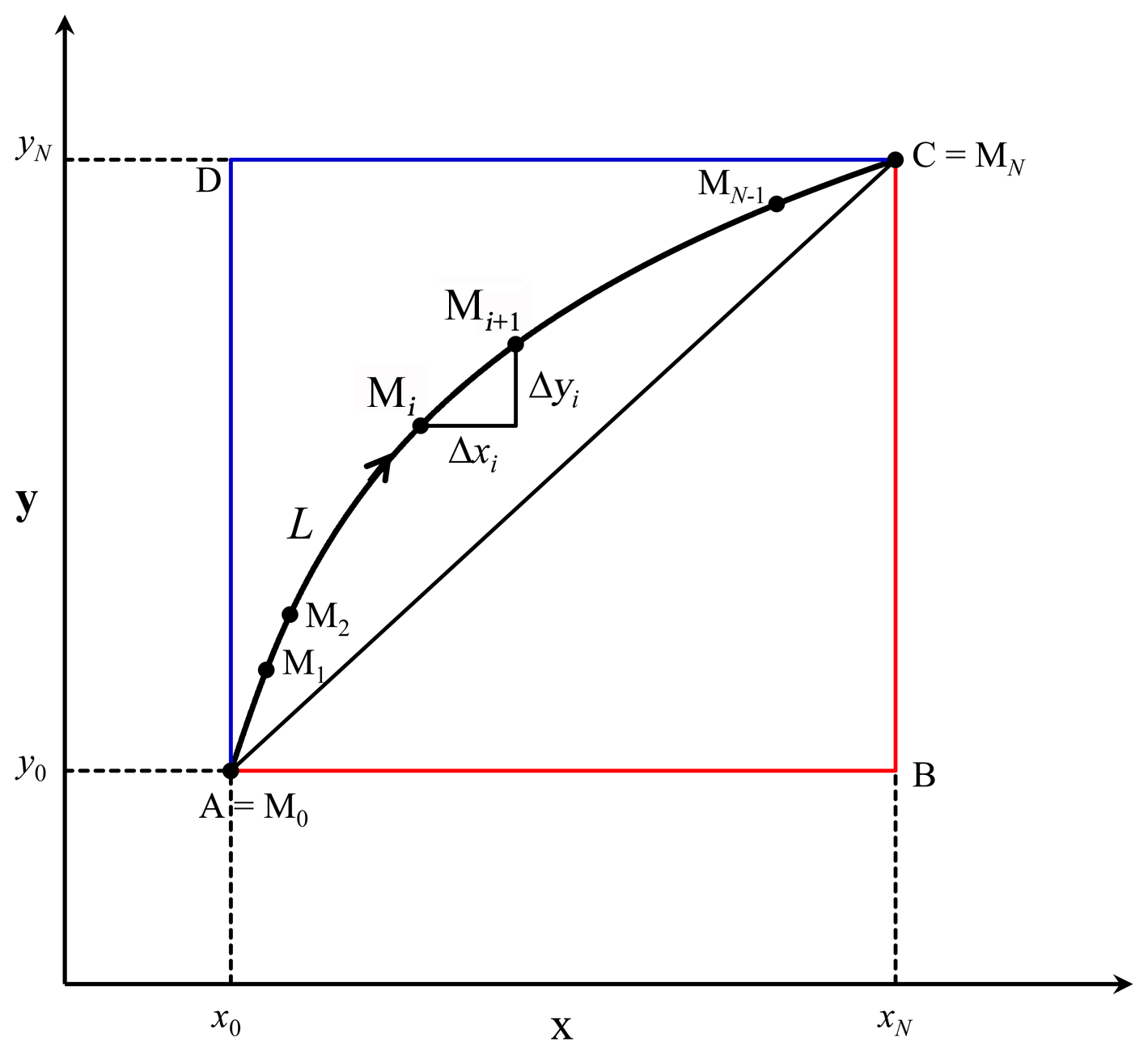
As shown in Fig. 3, points M1(x1,y1), …, partition L into N distinct segments. Let , , and . For each segment, Δzi can be approximated as dzi: . We then have . We thus obtain the following respective approximation of Δzx and Δzy: and . Next, define τ as the maximum length of the N segments. The smaller the value of τ, the closer the value of dzi is to Δzi and thus the more accurate the approximations are. The approximations become exact in the limit τ→0. Taking the limit τ→0 then converts the sum into integrals and gives a precise expression (this is an informal derivation; please see Appendix A for a formal one): , where and denote the line integral of fx and fy along L (termed integral path) with respect to x and y, respectively. and exist provided that fx and fy are continuous along L. We thus obtain a precise evaluation of Δzx and Δzy:
Unlike the total-differential method, the sum of Δzx and Δzy persistently equals Δz (Appendix B). If f(x,y) is linear, then fx and fy are constant. Let fx(x,y) and fy(x,y) remain constant at Cx and Cy, respectively; then Δzx=CxΔx and Δzy=CyΔy. Δzx and Δzy are thus independent of L. If f(x,y) is nonlinear, however, both Δzx and Δzy vary with L, as is exemplified in Appendix C. Hence, the initial and the terminal states, together with the path connecting them, determine the resultant partition unless f(x,y) is linear.
The mathematical derivation above applies to a three-variable function as well. By doing the line integrals for the MCY equation, we obtain the desired results:
where ΔRp, , and ΔRn denote the effects on runoff change of P, E0, and n, respectively. The sum of ΔRp and represents the effect of climate change, and ΔRn is often related to human activities although it probably includes the effects of other factors, such as climate seasonality (Roderick and Farquhar, 2011; Berghuijs and Woods, 2016). L denotes a three-dimensional curve along which climate and catchment changes have occurred. I approximated L by a series of line segments. ΔRp, , and ΔRn were finally determined by summing up the integrals along each of the line segments (see Sect. 2.3).
2.3 Using the LI method to determine ΔRp, , and ΔRn within the Budyko framework
-
Determining ΔRp, , and ΔRn assuming a linear integral path:
A curve can always be approximated as a series of line segments. Hence, we can first handle the case of a linear integral path. Given two consecutive periods and assuming that the catchment state has evolved from (P1, E01, n1) to (P2, E02, n2) along a straight line L, let , , and ; then the line L is given by parametric equations: , , , and . Given these equations, Eq. (2) becomes a univariate function of t, i.e., , , and . Then, ΔRP, , and ΔRn can be evaluated as
Unfortunately, I could not determine the antiderivatives of RP(t)dt, , and Rn(t)dt and had to make approximate calculations. As the discrete equivalent of integration is a summation, we can approximate the integration as a summation. I divided the interval into 1000 subintervals of the same width, i.e., setting dt identically equal to 0.001, and then calculated RP(t)dt, , and Rn(t)dt for each subinterval. Let ti=0.001i; and is integer-valued. ΔRp, , and ΔRn are approximated as
-
Dividing the evaluation period into a number of subperiods:
I first determined a change point and divided the whole observation period into the reference and evaluation periods. To determine the integral path, the evaluation period was further divided into a number of subperiods. The Budyko framework assumes a steady-state condition of a catchment and therefore requires no change in soil water storage. Over a time period of 5–10 years, it is reasonable to assume that changes in soil water storage will be sufficiently small (Zhang et al., 2001). Here, I divided the evaluation period into a number of 7-year subperiods with the exception for the final subperiod, which varied from 7 to 13 years in length depending on the length of the evaluation period.
-
Determining ΔRp, , and ΔRn by approximating the integral path as a series of line segments:
For a short period, the integral path L can be considered as linear, which implies a temporally invariant change rate. For a long period in which the change rate varies over time, L can be fitted using a number of line segments. Given a reference period and an evaluation period comprising N subperiods, the catchment state was assumed to evolve from (P0, E00, n0), …, (Pi, E0i, ni), …, to (PN, E0N, nN), where the subscript “0” denotes the reference period, and “i” and “N” denote the ith and the final subperiods of the evaluation period, respectively. I used a series of line segments L1, L2, …, LN to approximate the integral path L, where Li connects points (Pi−1, , ni−1) with (Pi, E0i, ni). Then ΔRp, , and ΔRn were evaluated as the sum of the integrals along each of the line segments, which were calculated using Eq. (6).
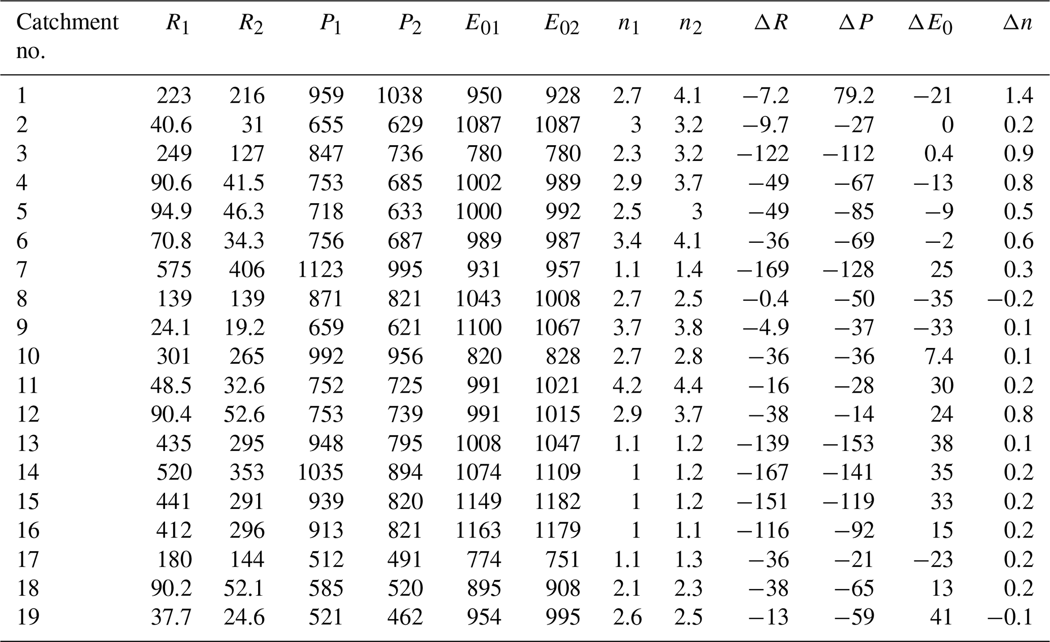
Table 1Summary of the long-term hydrometeorological characteristics of the selected catchmentsa.
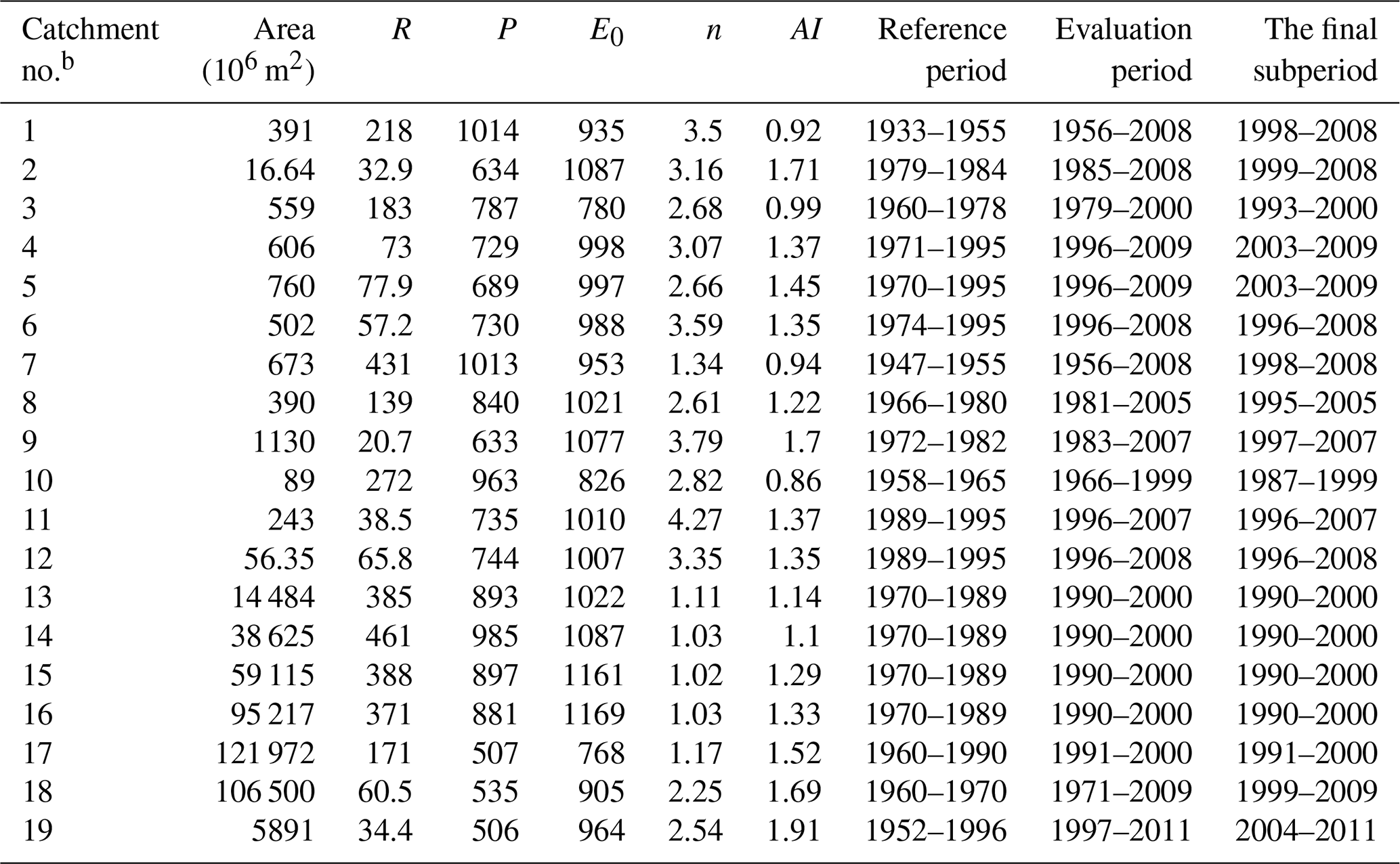
a R, P, and E0 represent the mean annual runoff, precipitation, and potential evaporation, all in 10−3m yr−1. n (dimensionless) is the parameter representing catchment properties in the MCY equation. AI is the dimensionless aridity index (). Data of catchments 1–12 were derived from Zhang et al. (2010). Data of catchments 13–16 were from Sun et al. (2014). Data of catchments 17, 18, and 19 were from Zheng et al. (2009), Jiang et al. (2015), and Gao et al. (2016), respectively. I used the change points given in the literatures to divide the observation period into the reference and elevation periods. The LI method further divides the evaluation period into a number of subperiods. The column “The final subperiod” denotes the final subperiod, which was used as the evaluation period for the total-differential method, the decomposition method, and the complementary method. b Catchments 1–12 are in Australia, and the others are in China. (1) Adjungbilly Creek; (2) Batalling Creek; (3) Bombala River; (4) Crawford River; (5) Darlot Creek; (6) Eumeralla River; (7) Goobarragandra Creek; (8) Jingellic Creek; (9) Mosquito Creek; (10) Traralgon Creek; (11) upper Denmark River; (12) Yate Flat Creek; (13) Yangxian station, Han River; (14) Ankang station, Han River; (15) Baihe station, Han River; (16) Danjiangkou station, Han River; (17) headwaters of the Yellow River basin; (18) Wei River; (19) Yan River.
2.4 Total-differential, decomposition, and complementary methods
To evaluate the LI method, I compared it with the existing methods, including the decomposition method, the total-differential method, and the complementary method. The total-differential method approximated ΔR as dR:
where , , and , representing the sensitivity coefficient of R with respect to P, E0, and n, respectively. Within the total-differential method,ΔRP=λPΔP, , and ΔRn=λnΔn. I used the forward approximation, i.e., substituting the observed mean annual values of the reference period into Eq. (2), to estimate λP, , and λn, as is standard in most studies (Roderick and Farquhar, 2011; Yang and Yang, 2011; Sun et al., 2014).
The decomposition method (Wang and Hejazi, 2011) calculated ΔRn as follows:
where R2, P2, and E2 represent the mean annual runoff, precipitation, and evapotranspiration of the evaluation period, respectively; R2′ and E2′ represent the mean annual runoff and evapotranspiration, respectively, given the climate conditions of the evaluation period and the catchment conditions of the reference period (Fig. 2). Both E2 and E2′ were calculated by Eq. (1) but using n values of the evaluation period and the reference period, respectively.
The complementary method (Zhou et al., 2016) uses a linear combination of the complementary relationship for runoff to determine ΔRp, , and ΔRn:
where the subscripts “1” and “2” denotes the reference and the evaluation periods, respectively. a is a weighting factor and varies from 0 to 1. As suggested by Zhou et al. (2016), I set a=0.5. Equation (9) thus gave an estimation of ΔRp, , and ΔRn as follows:
2.5 Data
I collected runoff and climate data from 19 selected catchments evaluated in previous studies (Table 1). The change-point years given in these studies were directly used to determine the reference and evaluation periods for the LI method. As mentioned above, the LI method further divides the evaluation period into a number of subperiods. For the sake of comparison, the final subperiod of the evaluation period was used as the evaluation period for the decomposition, the total-differential, and the complementary methods (it can be equally considered that all of the four methods used the final subperiod as the evaluation period, but the LI method cares about the intermediate period between the reference and the evaluation periods, and the other methods do not). Eight of the 19 catchments had a reference period comprising only one subperiod (Table 1), and the others had two to seven subperiods.
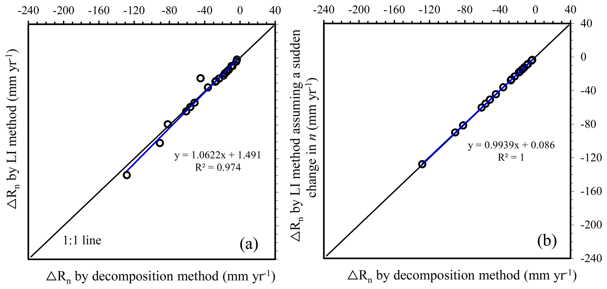
Figure 4Comparisons between the LI method and the decomposition method. (a) Comparison of the estimated contributions to the runoff changes from the catchment changes (ΔRn). (b) The decomposition method is equivalent to the LI method that assumes a sudden change in catchment properties following climate change. In this case, the integral path of the LI method can be considered as the path ABC in Fig. 3 (x represents climate factors, and y catchment properties, i.e., n) and , where the subscript “1” denotes the reference period and “2” denotes the final subperiod of the evaluation period.
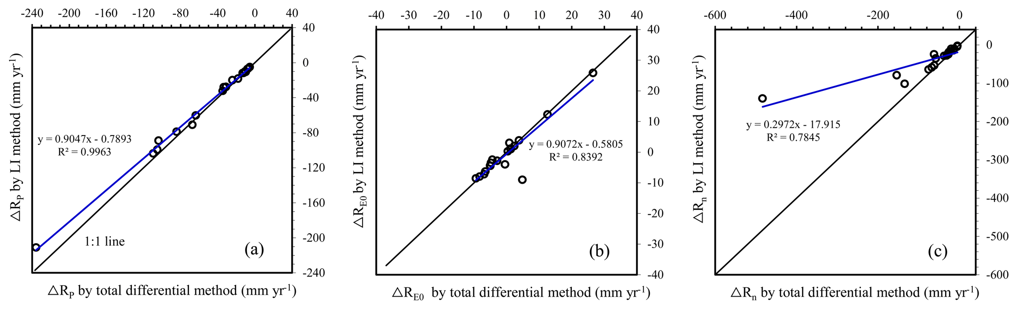
Figure 5Comparisons of the estimated contribution to runoff from the changes in (a) precipitation (ΔRP), (b) potential evapotranspiration (, and (c) catchment properties (ΔRn) between the LI method and the total-differential method.
The 19 selected catchments have diverse climates and landscapes, with 12 from Australia and seven from China (Table 1). The catchments span from tropical to subtropical and temperate areas and from humid to semi-humid and semiarid regions, with the mean annual rainfall varying from 506 to m and potential evaporation from 768 to m. The dryness index ranges between 0.86 and 1.91. The catchment areas vary by 5 orders of magnitude from 1.95 to 121 972 with a median 606×106 m2. The key data include annual runoff, precipitation, and potential evaporation. The record length varied between 19 and 76 with a median of 39 years. All the catchments experienced changes in climate and catchment properties over the observation periods. The precipitation changes from the reference to the evaluation period ranged between −153 and m yr−1, and between −35 and m yr−1 for potential evaporation (Table 2). The coeval change in the parameter n of the MCY equation ranged between −0.2 and 1.4. The mean annual streamflow reduced for all catchments, ranging from 0.4 to 169 with a median m yr−1. The change in catchment properties mainly refers to the vegetation cover or land use change. More details on the data and the catchments can be found in Zhang et al. (2010, 2011), Sun et al. (2014), Zheng et al. (2009), Jiang et al. (2015), and Gao et al. (2016).
Table 2Comparisons of R (mm yr−1), P (mm yr−1), E0 (mm yr−1), and n (dimensionless) between the reference and the evaluation periods*.
* The subscript “1” denotes the reference period, and ”2” denotes the evaluation period. (X as a substitute for R, P, E0, and n).
Table 3Effects of precipitation (ΔRP, 10−3 m yr−1), potential evapotranspiration (, 10−3 m yr−1), and catchment changes (ΔRn, 10−3 m yr−1) on the mean annual runoff determined from the four evaluated methods.

Table 3 lists the resultant values of ΔRp, , and ΔRn from the LI method and the three other methods. Please see the Supplement for detailed calculation steps.
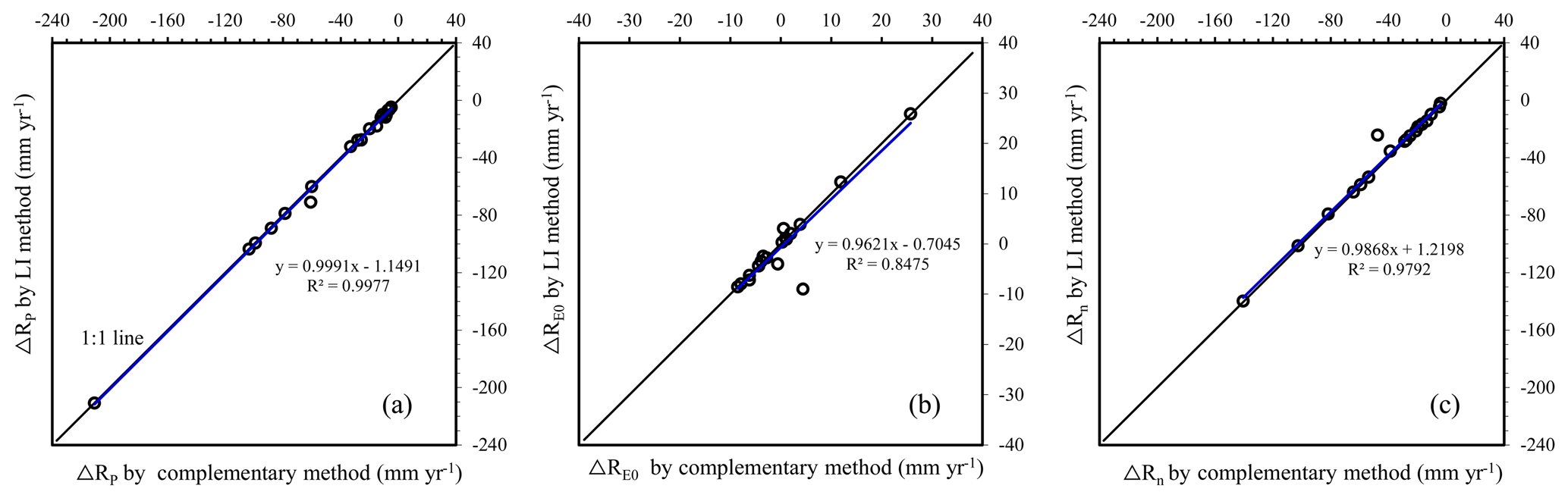
Figure 6Comparisons of (a) ΔRP, (b) , and (c) ΔRn between the LI method and the complementary method (a=0.5).
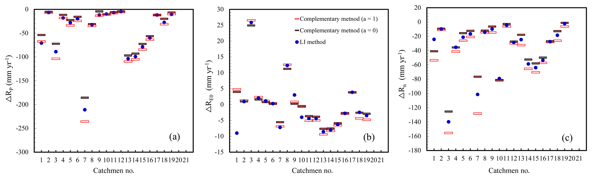
Figure 7Comparisons of (a) ΔRP, (b) , and (c) ΔRn by the LI method with the upper and lower bounds given by the complementary method. According to Zhou et al. (2016), ΔRP, , and ΔRn reach their bounds when a is 0 or 1.
Figure 4a compares the resultant ΔRn of the LI method and the decomposition method. Although they are quite similar, the discrepancies can be m yr−1. The decomposition method assumes that climate change occurs first and then human interferences cause a sudden change in catchment properties (Fig. 2). Such a fictitious path is identical to the path ABC in Fig. 3, provided that x represents climate factors and y catchment properties. When ABC was adopted as the integral path, the LI method yielded the same results as the decomposition method did (Fig. 4b). Hence, the decomposition method can be considered as a case of the LI method that uses a special integral path.
The total-differential method is predicated on an approximate equation, i.e., Eq. (7). The LI method reveals that the precise form of the equation is (Appendix D), where , , and denote the path-averaged sensitivity of R to P, E0, and n, respectively. All points along the path have the same weight in determining , , and . To determine them, the total-differential and the complementary methods utilize only the initial and/or the terminal states. Neglecting the intermediate states results in an imprecise partition, as was illustrated in Figs. 5 and 6 as well as in Fig. 1 using a univariate function, and even a reverse trend estimation (see for catchment no. 1 in Table 3).
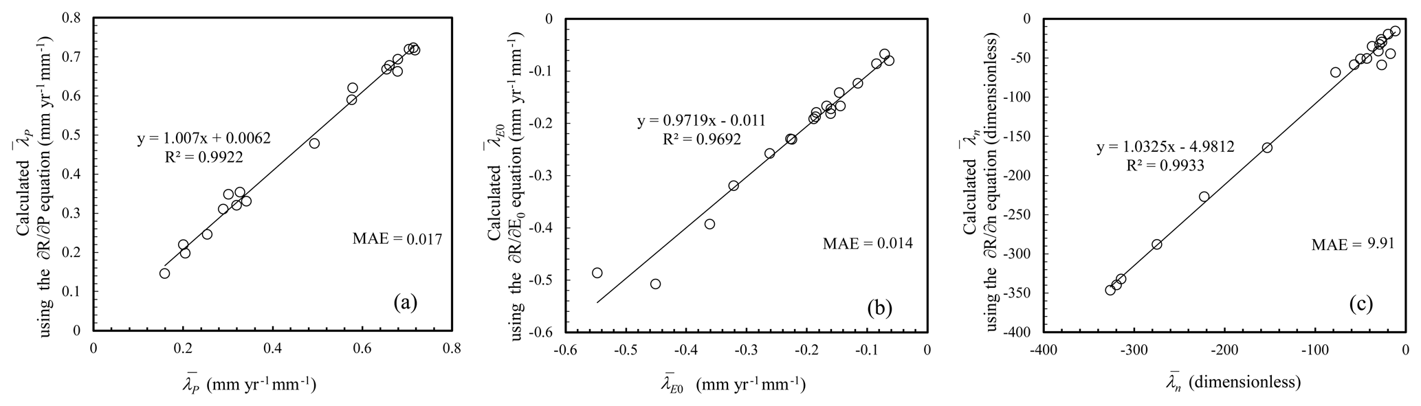
Figure 8Performances of Eq. (2) to be used to predict , , and with the long-term mean values of P, E0, and n as inputs. is the mean absolute error, where O and P are values that were actually encountered (given in Table S4) and predicted using Eq. (2), respectively, and N is the number of selected catchments.
As with the LI method, the complementary method produced ΔRP, , and ΔRn that exactly summed up to ΔR. Although its resultant ΔRp, , and ΔRn values were all in accordance with the LI method (Fig. 6), the LI method often yielded values beyond the bounds given by the complementary method (Fig. 7); this is because the maximum or minimum sensitivities do not necessarily occur at the initial or terminal states.
, and imply the average runoff change induced by a unit change in P, E0, and n, respectively (Appendix D). , , and all varied by up to several times or even 10-fold between the studied catchments (Table S4). Figure 8 shows that Eq. (2) reproduced , , and very well when taking the long-term means of P, E0, and n as inputs, a reflection of the fact that the dependent variable approached its average when the independent variables were set to be their averages. This finding is of relevance to the spatial prediction of , , and .
The LI method highlights the role of the evolutionary path in determining the resultant partition. Yet it seems that no studies have accounted for the path issue while evaluating the relative influences of drivers. The limit of the LI method is high data requirements for obtaining the evolutionary path. When the path data are unavailable, the complementary method can be considered as an alternative. The complementary method is free of residuals; moreover, it employs data from both the reference and the evaluation periods, thereby generally yielding sensitivities closer to the path-averaged results than the total-differential method.
While using the Budyko models, a reasonable timescale is relevant to meet the assumption that changes in catchment water storage are small relative to the magnitude of fluxes of P, R, and E (Donohue et al., 2007; Roderick and Farquhar, 2011). A 7-year timescale was used in the present study, as most studies have suggested that a time period of 5–10 years (Zhang et al., 2001, 2016; Wu et al., 2017a, b; Li et al., 2017) or even 1 year (Roderick and Farquhar, 2011; Sivapalan et al., 2011; Carmona et al., 2014; Ning et al., 2017) is reasonable. Nevertheless, some studies have argued that the time period should be longer than 10 years (Li et al., 2016; Dey and Mishra, 2017). Using the Gravity Recovery and Climate Experiment (GRACE) satellite gravimetry, Zhao et al. (2011) detected the water storage variations for the three largest river basins of China, namely, the Yellow, Yangtze, and Zhujiang. The Yellow River mostly drains an arid and semiarid region (P, m; R, m; E, m), and the Yangtze (P, m; R, m; E, m) and the Zhujiang River basins (P, m; R, m; E, m) are humid. The amplitude of the water storage variations between years was 7, 37.2, and m for the three rivers, respectively, at 1 order of magnitude smaller than the fluxes of P, R and E. Although the observations cannot be directly extrapolated to other regions, the possibility seems remote that the use of a 7-year aggregated time period strongly violates the assumption of the steady-state condition.
The mutual independence of the drivers is crucial for a valid partition. In the present study, although annual P and E0 exhibited significant correlation for most catchments (p<0.05), the aggregated P, E0, and n over a 7-year period showed minimal correlation (mostly p>0.1). The interdependence between the drivers can considerably confound the resultant partitions of the LI method and other existing methods.
The LI method revises the concept of sensitivity at a point as the path-averaged sensitivity. Mathematically, the LI method is unrelated to a functional form and hence applies to communities other than just hydrology. For example, identifying the carbon emission budgets (an allowable amount of anthropogenic CO2 emission consistent with a limiting warming target) is crucial for global efforts to mitigate climate change. The LI method suggested that the emission budgets depends on both the emission magnitude and pathway (timing of emissions), which is in line with a recent study by Gasser et al. (2018). An optimal pathway would facilitate an elevated carbon budget unless the carbon–climate system behaves in a linear fashion.
This study presented the LI method using time-series data, but it applies equally to the case of spatial series of data. Given a model that relates fluvial or eolian sediment load to the influencing factors (e.g., rainfall and topography), for example, the LI method can be used to separate their contributions to the sediment-load change along a river or in the along-wind direction.
Based on the line integral, I created a mathematically precise method to partition the synergistic effects of several factors that cumulatively drive a system to change from one state to the other. The method is relevant for quantitative assessments of the relative roles of the factors behind the change in the system state. I applied the LI method to partition the effects of climatic and catchment conditions on runoff within the Budyko framework. The method reveals that, in addition to the change magnitude, the change pathways of climatic and catchment conditions also play a role. Instead of using the runoff sensitivity at a point, the LI method uses the path-averaged sensitivity, thereby ensuring a mathematically precise partition. As a mathematically accurate scheme, the LI method has the potential to be a generic attribution approach in the environmental sciences.
Proof. In order to prove the equation above, we define the curve L in Fig. 3 as being given by a parametric equation: x=x(t), y=y(t), , and therefore . Substituting the parametric
equations, the right-hand side of the equation can be rewritten as
Let , and after using the chain rule to differentiate g with respect to t we obtain
Thus, g′(t) is just the integrand in Eq. (A1), and the right-hand side of the equation can be further rewritten as follows.
The right-hand side of the equation the left-hand side of the equation. Q.E.D.
Preliminary theorem: Given an open, simply connected region G (i.e., no holes in G) and two functions P(x,y) and Q(x,y) that have continuous first-order derivatives, if and only if throughout G, then is path independent; i.e., it depends solely on the starting and ending points of L.
Proof. We have and . As , we can state that , meeting the above condition and proving that is path independent. The statement was further exemplified using a fictitious example in Appendix C. Q.E.D.
Runoff (R, 10−3 m yr−1) at a site is assumed to increase from 120 to m yr−1 with m yr−1; meanwhile, precipitation (P, 10−3 m yr−1) varies from 600 to m yr−1 ( m yr−1) and the runoff coefficient (CR, dimensionless) varies from 0.2 to 0.3 (ΔCR=0.1). The goal is to partition ΔR into the effects of the precipitation (ΔRP) and runoff coefficient (), provided that P and CR are independent. We have a function R=PCR and its partial derivatives and . Given a path L along which P and CR change and using Eq. (3), the LI method evaluates ΔRP and as
The result differs depending on L, but the sum of ΔRP and uniformly equals ΔR. This dynamic is demonstrated using Fig. 3, in which we considered that the x axis represents CR, and the y axis P. Point A denotes the initial state (CR=0.2, P=600), and point C the terminal state (CR=0.3, P=650). I calculated ΔRP and along three fictitious paths as follows:
-
L= AC. Line segment AC has equation , . Let us take CR as the parameter and write the equation in the parametric form as , CR=CR, . By substituting the equation into Eq. (C1), we have
-
L= AB + BC. To evaluate on the broken line, we can evaluate separately on AB and BC and then sum them up. The equation for AB is P=600, , while for BC it is CR=0.3, . Note that a constant CR or P implies that dCR=0 or dP=0. Eq. (C1) then becomes
-
. The equation for AD is CR=0.2, , and for DC it is P=650, . ΔRP and are evaluated as
As expected, the sum of ΔRP and persistently equals ΔR although ΔRP and varies with L.
If the interval [x0, xN] in Fig. 3 is partitioned into N distinct bins of the same width , Eq (3a) can then be rewritten as
where , denoting the average of fx(x, y) along the curve L. Likewise, we have , where denotes the average of fy(x,y) along the curve L. As a result
The result can readily be extended to a function of three variables. Applying the mathematic derivation determined above to the MCY equation results in a precise form of Eq. (7):
where ; ; ; and , , and denote the arithmetic mean of , , and along a path of climate and catchment changes, respectively. Because , , and , , , and also imply the runoff change due to a unit change in P, E0, and n, respectively.
Given a one-dimensional function z=f(x) and its derivative f′(x), we assumed that f′(x) averages over the range , i.e., . According to the mean value theorem for integrals, . In terms of the Newton–Leibniz formula, . Thus, we obtain .
The data used in this study are freely available by contacting the author.
The supplement related to this article is available online at: https://doi.org/10.5194/hess-24-2365-2020-supplement.
MZ designed the study, analyzed the data, and wrote the manuscript.
The author declares that there is no conflict of interest.
I thank Yuanqiong Zheng for his assistance with the mathematical proof in Appendix A.
This research has been supported by the National Natural Science Foundation of China (grant no. 41671278) and the Guangdong Academy of Sciences' Project of Science and Technology Development (grant nos. 2019GDASYL-0103043, 2019GDASYL-0502004, 2019GDASYL-0401003, 2019GDASYL-0301002, 2019GDASYL-0503003, and 2019GDASYL-0102002).
This paper was edited by Erwin Zehe and reviewed by two anonymous referees.
Barnett, T. P., Pierce, D. W., Hidalgo, H. G., Bonfils, C., Santer, B. D., Das, T., .Bala G., Woods, A. W., Nozawa, T., Mirin, A. A., Cayan D. R., and Dettinger, M. D.: Human-induced changes in the hydrology of the western United States, Science, 319, 1080–1083, https://doi.org/10.1126/science.1152538, 2008.
Berghuijs, W. R., and Woods, R. A.: Correspondence: Space-time asymmetry undermines water yield assessment, Nat. Commun., 7, 11603, https://doi.org/10.1038/ncomms11603, 2016.
Binley, A. M., Beven, K. J., Calver, A., and Watts, L. G.: Changing responses in hydrology: assessing the uncertainty in physically based model predictions, Water Resour. Res., 27, 1253–1261, https://doi.org/10.1029/91WR00130, 1991.
Brown, A. E., Zhang, L., McMahon, T. A., Western, A. W., and Vertessy, R. A.: A review of paired catchment studies for determining changes in water yield resulting from alterations in vegetation, J. Hydrol., 310, 26–61, https://doi.org/10.1016/j.jhydrol.2004.12.010, 2005.
Budyko, M. I.: Climate and Life, Academic, NY, 508 pp., 1974.
Carmona, A. M., Sivapalan, M., Yaeger, M. A., and Poveda, G.: Regional patterns of interannual variability of catchment water balances across the continental US: A Budyko framework, Water Resour. Res., 50, 9177–9193, https://doi.org/10.1002/2014wr016013, 2014.
Choudhury, B. J.: Evaluation of an empirical equation for annual evaporation using field observations and results from a biophysical model, J. Hydrol., 216, 99–110, https://doi.org/10.1016/S0022-1694(98)00293-5, 1999.
Dey, P. and Mishra, A.: Separating the impacts of climate change and human activities on streamflow: A review of methodologies and critical assumptions, J. Hydrol., 548, 278–290, https://doi.org/10.1016/j.jhydrol.2017.03.014, 2017.
Donohue, R. J., Roderick, M. L., and McVicar, T. R.: On the importance of including vegetation dynamics in Budyko's hydrological model, Hydrol. Earth Syst. Sci., 11, 983–995, https://doi.org/10.5194/hess-11-983-2007, 2007.
Gao, G., Ma, Y., and Fu, B.: Multi-temporal scale changes of streamflow and sediment load in a loess hilly watershed of China, Hydrol. Process., 30, 365–382, https://doi.org/10.1002/hyp.10585, 2016.
Gasser, T., Kechiar, M., Ciais, P., Burke, E. J., Kleinen, T., Zhu, D., Huang, Y., Ekici, A., and Obersteiner, M.: Path-dependent reductions in CO2 emission budgets caused by permafrost carbon release, Nat. Geosci., 11, 830–835, https://doi.org/10.1038/s41561-018-0227-0, 2018.
Jiang, C., Xiong, L., Wang, D., Liu, P., Guo, S., and Xu C.: Separating the impacts of climate change and human activities on runoff using the Budyko-type equations with time-varying parameters, J. Hydrol., 522, 326–338, https://doi.org/10.1016/j.jhydrol.2014.12.060, 2015.
Li, Z., Ning, T., Li, J., and Yang, D.: Spatiotemporal variation in the attribution of streamflow changes in a catchment on China's Loess Plateau, Catena, 158, 1–8, https://doi.org/10.1016/j.catena.2017.06.008, 2017.
Liang, W., Bai, D., Wang, F., Fu, B., Yan, J., Wang, S., Yang, Y., Long, D., and Feng, M.: Quantifying the impacts of climate change and ecological restoration on streamflow changes based on a Budyko hydrological model in China's Loess Plateau, Water Resour. Res., 51, 6500–6519, https://doi.org/10.1002/2014WR016589, 2015.
Mezentsev, V. S.: More on the calculation of average total evaporation, Meteorol. Gidrol., 5, 24–26, 1955.
Ning, T., Li, Z., and Liu, W.: Vegetation dynamics and climate seasonality jointly control the interannual catchment water balance in the Loess Plateau under the Budyko framework, Hydrol. Earth Sys. Sci., 21, 1515–1526, https://doi.org/10.5194/hess-2016-484, 2017.
Roderick, M. L. and Farquhar, G. D.: A simple framework for relating variations in runoff to variations inclimatic conditions and catchment properties, Water Resour. Res., 47, W00G07, https://doi.org/10.1029/2010WR009826, 2011.
Sankarasubramanian, A., Vogel, R. M., and Limbrunner, J. F.: Climate elasticity of streamflow in the United States, Water Resour. Res., 37, 1771–1781, https://doi.org/10.1029/2000WR900330, 2001.
Schaake, J. C.: From climate to flow, Climate Change and U.S. Water Resources, edited by: Waggoner, P. E., chap. 8, John Wiley, NY, 177–206, 1990.
Sivapalan, M., Yaeger, M. A., Harman, C. J., Xu, X. Y., and Troch, P. A.: Functional model of water balance variability at the catchment scale: 1. Evidence of hydrologic similarity and space-time symmetry, Water Resour. Res., 47, W02522, https://doi.org/10.1029/2010wr009568, 2011.
Sposito, G.: Understanding the Budyko equation, Water, 9, 236, https://doi.org/10.3390/w9040236, 2017.
Sun, Y., Tian, F., Yang, L., and Hu, H.: Exploring the spatial variability of contributions from climate variation and change in catchment properties to streamflow decrease in a mesoscale basin by three different methods, J. Hydrol., 508, 170–180, https://doi.org/10.1016/j.jhydrol.2013.11.004, 2014.
Wang, D. and Hejazi, M.: Quantifying the relative contribution of the climate and direct human impacts on mean annual streamflow in the contiguous United States, Water Resour. Res., 47, W00J12, https://doi.org/10.1029/2010WR010283, 2011.
Wang, W., Shao, Q., Yang, T., Peng, S., Xing, W., Sun, F., and Luo, Y.: Quantitative assessment of the impact of climate variability and human activities on runoff changes: A case study in four catchments of the Haihe River basin, China, Hydrol. Process., 27, 1158–1174, https://doi.org/10.1002/hyp.9299, 2013.
Wu, J., Miao, C., Wang, Y., Duan, Q., and Zhang, X.: Contribution analysis of the long-term changes in seasonal runoff on the Loess Plateau, China, using eight Budyko-based methods, J. Hydrol., 545, 263–275, https://doi.org/10.1016/j.jhydrol.2016.12.050, 2017a.
Wu, J., Miao, C., Zhang, X., Yang, T., and Duan, Q.: Detecting the quantitative hydrological response to changes in climate and human activities, Sci. Total Environ., 586, 328–337, https://doi.org/10.1016/j.scitotenv.2017.02.010, 2017b.
Xu, X., Yang, D., Yang, H., and Lei, H.: Attribution analysis based on the Budyko hypothesis for detecting the dominant cause of runoff decline in Haihe basin, J. Hydrol., 510, 530–540, https://doi.org/10.1016/j.jhydrol.2013.12.052, 2014.
Yang, H. and Yang, D.: Derivation of climate elasticity of runoff to assess the effects of climate change on annual runoff, Water Resour. Res., 47, W07526, https://doi.org/10.1029/2010WR009287, 2011.
Yang, H., Yang, D., Lei, Z., and Sun, F.: New analytical derivation of the mean annual water-energy balance equation, Water Resour. Res., 44, W03410, https://doi.org/10.1029/2007WR006135, 2008.
Yang, H., Yang, D., and Hu, Q.: An error analysis of the Budyko hypothesis for assessing the contribution of climate change to runoff, Water Resour. Res., 50, 9620–9629, https://doi.org/10.1002/2014WR015451, 2014.
Zhang, L., Dawes, W. R., and Walker, G. R.: Response of mean annual evapotranspiration to vegetation changes at catchment scale, Water Resour. Res., 37, 701–708, https://doi.org/10.1029/2000WR900325, 2001.
Zhang, L., Zhao, F., Brown, A., Chen, Y., Davidson, A., and Dixon, R.: Estimating Impact of Plantation Expansions on Streamflow Regime and Water Allocation, CSIRO Water for a Healthy Country, Canberra, Australia, 1–69, 2010.
Zhang, L., Zhao, F., Chen, Y., and Dixon, R. N. M.: Estimating effects of plantation expansion and climate variability on streamflow for catchments in Australia, Water Resour. Res., 47, W12539, https://doi.org/10.1029/2011WR010711, 2011.
Zhang, S., Yang, H., Yang, D., and Jayawardena, A. W.: Quantifying the effect of vegetation change on the regional water balance within the Budyko framework, Geophys. Res. Lett., 43, 1140–1148, https://doi.org/10.1002/2015GL066952, 2016.
Zhao, Q. L., Liu, X. L., Ditmar, P., Siemes, C., Revtova, E., Hashemi-Farahani, H., and Klees, R.: Water storage variations of the Yangtze, Yellow, and Zhujiang river basins derived from the DEOS Mass Transport (DMT-1) model, Sci. China-Earth Sci., 54, 667–677, https://doi.org/10.1007/s11430-010-4096-7, 2011.
Zheng, H., Zhang, L., Zhu, R., Liu, C., Sato, Y., and Fukushima, Y.: Responses of streamflow to climate and land surface change in the headwaters of the Yellow River Basin, Water Resour. Res., 45, W00A19, https://doi.org/10.1029/2007WR006665, 2009.
Zhou, S., Yu, B., Zhang, L., Huang, Y., Pan, M., and Wang, G.: A new method to partition climate and catchment effect on the mean annual runoff based on the Budyko complementary relationship, Water Resour. Res., 52, 7163–7177, https://doi.org/10.1002/2016WR019046, 2016.
- Abstract
- Introduction
- Methodology
- Results
- Discussion
- Conclusions
- Appendix A: Mathematical proof of
- Appendix B: Mathematical proof that the sum of and is path independent
- Appendix C: A fictitious example to show how the LI method works
- Appendix D: Mathematical proof of the path-averaged sensitivity
- Appendix E: Path-averaged sensitivity in one-dimensional cases
- Data availability
- Author contributions
- Competing interests
- Acknowledgements
- Financial support
- Review statement
- References
- Supplement