Should altitudinal gradients of temperature and precipitation inputs be inferred from key parameters in snow-hydrological models?

Ruelland, Denis

doi:https://doi.org/10.5194/hess-24-2609-2020

Articles | Volume 24, issue 5

https://doi.org/10.5194/hess-24-2609-2020

Articles | Volume 24, issue 5

Research article

20 May 2020

Research article |

| 20 May 2020

Should altitudinal gradients of temperature and precipitation inputs be inferred from key parameters in snow-hydrological models?

Denis Ruelland

Abstract

This paper evaluates whether snow-covered area and streamflow measurements can help assess altitudinal gradients of temperature and precipitation in data-scarce mountainous areas more efficiently than using the usual interpolation procedures. A dataset covering 20 Alpine catchments is used to investigate this issue. Elevation dependency in the meteorological fields is accounted for using two approaches: (i) by estimating the local and time-varying altitudinal gradients from the available gauge network based on deterministic and geostatistical interpolation methods with an external drift; and (ii) by calibrating the local gradients using an inverse snow-hydrological modelling framework. For the second approach, a simple two-parameter model is proposed to target the temperature/precipitation–elevation relationship and to regionalize air temperature and precipitation from the sparse meteorological network. The coherence of the two approaches is evaluated by benchmarking several hydrological variables (snow-covered area, streamflow) computed with snow-hydrological models fed with the interpolated datasets and checked against available measurements. Results show that accounting for elevation dependency from scattered observations when interpolating air temperature and precipitation cannot provide sufficiently accurate inputs for models. The lack of high-elevation stations seriously limits correct estimation of lapse rates of temperature and precipitation, which, in turn, affects the performance of the snow-hydrological simulations due to imprecise estimates of temperature and precipitation volumes. Instead, retrieving the local altitudinal gradients using an inverse approach enables increased accuracy in the simulation of snow cover and discharge dynamics while limiting problems of over-calibration and equifinality.

Download & links

Article (PDF, 6965 KB)

How to cite

How to cite.

Dates

Received: 17 Oct 2019 – Discussion started: 12 Nov 2019 – Revised: 19 Apr 2020 – Accepted: 23 Apr 2020 – Published: 20 May 2020

1 Introduction

1.1 Providing accurate meteorological inputs in mountainous regions

Regionalizing air temperature and precipitation is a critical step in producing accurate areal inputs for hydrological models in high-altitude catchments. The ability to correctly reproduce areal precipitation is essential to avoid the failure of hydrological models, which are sensitive to input volumes at the catchment scale (e.g. Oudin et al., 2006; Nicótina et al., 2008). Accurate temperature fields are also particularly important in mountainous regions because temperature is the main driver of snow–rain partition and snowmelt and consequently influences seasonal discharge (e.g. Hublart et al., 2015, 2016).

However, in areas with complex topography, the characteristic spatial scales of temperature and precipitation estimates are typically poorly captured, notably when the network of measurements used is sparse. Gridded datasets obtained by interpolating measurements taken at meteorological stations are thus affected by inaccuracies, which are spatially and temporally variable and difficult to quantify (Haylock et al., 2008; Isotta et al., 2014). Measurement errors depend on local conditions and increase with terrain elevation as the operational conditions become more extreme (Frei and Schär, 1998). In the case of precipitation, a well-known problem arises from the systematic errors associated with precipitation under-catch during snowfall (Strasser et al., 2008), especially in windy conditions (Sevruk, 2005). In addition, temperature and precipitation are under-sampled at high elevations, because meteorological stations are mainly located at low elevations for logistical reasons (Hofstra et al., 2010). This makes it difficult to derive the local and seasonal relationship between meteorological observations and topography, even though this is indispensable for accurate spatial temperature and precipitation estimates (Masson and Frei, 2014). Indeed, atmospheric uplift caused by relief tends to increase precipitation with elevation through the so-called orographic effect (Barry and Chorley, 2010). Nevertheless, precipitation accumulation trends can show considerable scatter with altitude depending on the region's exposure to wind and synoptic situations (Sevruk, 1997). The relationship between temperature and elevation is generally more obvious. The rate at which air cools with a change in elevation ranges from about −0.98 ^∘C (100 m)⁻¹ for dry air (i.e. the dry-air adiabatic lapse rate) to about −0.40 ^∘C (100 m)⁻¹ (i.e. the saturated adiabatic lapse rate; Dodson and Marks, 1997). Average temperature gradients of −0.60 ^∘C (Dodson and Marks, 1997) or −0.65 ^∘C (100 m)⁻¹ (Barry and Chorley, 2010) are often used when high precision is not required. However, such average values are known to be rough approximations which are not suitable for more precise studies (see e.g. Douguédroit and De Saintignon, 1984). Notably they mask significant variations in different meteorological conditions and in different seasons. For instance, temperature lapse rates are generally lower in winter than in summer, as shown by Rolland (2003) for Alpine regions.

1.2 Schemes for spatial interpolation of air temperature or precipitation

The mapping of air temperature and precipitation using discrete observations based on gauge networks has been extensively studied. Readers can refer to, for instance, Ly et al. (2013) for a review of the different deterministic and geostatistical methods designed for operational hydrology and hydrological modelling at the catchment scale.

Schemes for spatial interpolation of meteorological variables vary in three ways (Stahl et al., 2006): (1) the model used to characterize the spatial variation of the variable of interest, (2) the method used to choose the surrounding points (number or distance, angular position relative to the prediction point), and (3) the approach used to adjust for elevation. The simplest approach is to choose the nearest station and adjust for elevation according to an assumed lapse rate. However, this method is fairly crude and ignores fine-scale spatial variations. Where more than one station is used in the prediction, a model is required to determine how to interpolate from them. Interpolation weights have been estimated using approaches including inverse distance weighting (IDW) (e.g. Dodson and Marks, 1997; Shen et al., 2001; Frei, 2014) and geostatistical methods based on kriging (e.g. Garen and Marks, 2005; Spadavecchia and Williams, 2009). Kriging relies on statistical models involving autocorrelation, which refers to the statistical relationships between measured points. Ordinary kriging (OKR) is well-known among kriging algorithms (see e.g. Goovaerts (2000) for a detailed presentation of these algorithms). Different methods have been developed to deal with the statistical relationship between temperature/precipitation and elevation, like regression analysis (Drogue et al., 2002) or more elaborate geostatistical techniques including simple kriging with local means, kriging with external drift (KED), and co-kriging (CKR): see Goovaerts (2000) for a comparison of these approaches. Among these techniques, KED has been widely used to generate temperature and precipitation maps. For instance, Masson and Frei (2014) showed that KED led to much smaller interpolation errors than linear regressions in the Alps. This was achieved with a single predictor (local topographic height), whereas the incorporation of more extended predictor sets (slope, circulation-type dependence of the relationship, inclusion of a wind-aligned predictor) enabled only marginal improvement. For daily precipitation, interpolation accuracy improved considerably with KED and the use of a simple digital elevation compared to OKR (i.e. with no predictor). These results confirm that accounting for topography is important for spatial interpolation of daily precipitation in high-mountain regions. Conversely, other authors showed that, even though taking topography into account was indispensable for temperature reconstruction whatever the temporal resolution, it was less clear for daily precipitation. For example, Ly et al. (2011) reported no improvement in precipitation estimated at a daily timescale if topographical information was taken into account with KED and CKR, compared to simpler methods such as ORK and IDW. In a recent and very complete comparative study, Berndt and Haberlandt (2018) analysed the influence of temporal resolution and network density on the spatial interpolation of climate variables. They showed that KED using elevation performed significantly better than ORK for temperature data at all temporal resolutions and station densities. For precipitation, using elevation as additional information in KED improved the interpolation performance at the annual timescale, but not at the daily timescale.

Theoretically, KED can account for local differences in topographic influence in different seasons and synoptic situations. Indeed, the regression coefficients computed between the primary variable (temperature or precipitation) and the secondary variable (elevation) are implicitly estimated through the kriging system within each search neighbourhood (Goovaerts, 2000). The relation between variables is thus assessed locally, meaning changes in correlation across the study area can be taken into account. However, as suggested by Stahl et al. (2006) concerning temperature and by Ly et al. (2011) concerning precipitation, care should be taken in applying KED when interpolating daily variables with very few neighbouring sample points. Indeed, methods that compute local lapse rates from the surrounding control points can perform poorly in regions with insufficient high-elevation data, due to inaccurate estimation of local lapse rates.

1.3 Placing meteorological fields in a hydrological perspective

A subject that requires further investigation is which methods that produce daily temperature and precipitation fields can provide the best snow-cover and streamflow simulations. The usual cross-validation for the inter-comparison of interpolation methods is limited, especially in ungauged areas like the highest parts of mountainous areas. As stressed by Gottardi et al. (2012), a method can perform well in interpolation (at the ground network altitudes) but poorly in extrapolation (higher). This is because the observed set is not representative of the entire feature space. As a result, estimations at high elevations are difficult to check due to the lack of meteorological data. To go further, the use of other data like streamflow measurements may be a good alternative way to validate temperature and precipitation estimations at high-elevation sites.

To date, few studies have compared the performance of different interpolation methods evaluated by hydrological modelling in mountainous areas. Among the few that have, Tobin et al. (2011) showed that kriging (and more specifically KED) can be used effectively to estimate temperature and precipitation fields in complex Alpine topography during flood events. Their comparative analyses of the different interpolation techniques suggested that geostatistical methods performed better than IDW. In particular, with elevation as auxiliary information, KED gave the overall best validation statistics for the set of events under study. However, it can be hypothesized that, in many mountainous areas, gauge observations do not include sufficient information to accurately account for the elevation dependency of air temperature and precipitation using interpolation techniques, which are thus limited to providing accurate inputs for snow-hydrological models. On the other hand, numerous calibration parameters controlling snow accumulation (the temperature threshold between the solid and liquid phases, temperature range of phase separation, snowfall gauge under-catch factor) and snowmelt (temperature threshold for snowmelt, degree-day melt factor, snowpack thermal state, etc.) have been introduced in most of the snow accounting routines (SARs) used in operational hydrology: see e.g. HBV (Bergström, 1975), MOHYSE (Fortin and Turcotte, 2006), CEMANEIGE (Valéry et al., 2014), and MORDOR (Garavaglia et al., 2017). The aim of using these parameters is to adapt to local snow processes, but they could be used primarily to compensate for errors in the input data without satisfactorily achieving it.

1.4 Inverting the hydrological cycle

In contrast, inverting the hydrological cycle with snow-hydrological models may help identify the dependency of the areal inputs on elevation more realistically and enable more accurate snow-hydrological simulations while simultaneously limiting the number of free parameters. The idea is not completely new and was notably introduced by Valéry et al. (2009) in an attempt to use streamflow measurements to improve knowledge of yearly precipitation in data-sparse mountainous regions. Their results suggested that it was possible to unambiguously identify the altitudinal precipitation gradients from streamflow at a yearly timescale. In another paper, Valéry et al. (2010) proposed regionalization of daily air temperature and precipitation to better estimate inputs over high-altitude catchments as regards to the water balance. In their conclusion, the authors claimed that their regionalization approach also significantly improved the performance of a rainfall-runoff model at a daily timescale. However, the lapse rates in the temperature and precipitation inputs were estimated from gauge observations at the regional scale based on a leave-one-out procedure. This leaves room for potential improvement by locally inferring the lapse rates based on inverse modelling applied at the catchment scale.

A few studies proposed approaches to estimate lapse rates based on hydrological modelling in specific catchments. Zhang et al. (2015) showed that the runoff simulation results involving snowmelt and rainfall runoff were highly sensitive to the temperature and precipitation lapse rates in a Tibetan catchment. Rahman et al. (2014) calibrated the SWAT model in a snow-dominated basin in the Swiss Alps and found also that the temperature lapse rate was significantly important for hydrological performance. Naseer et al. (2019) considered a dynamic lapse rate based on a vertical profile of temperature in a catchment in Japan and succeeded in improving the precipitation phase in a distributed hydrological modelling framework. Henn et al. (2016) investigated the value of snow data to constrain the inference of precipitation from streamflow, using lumped hydrologic models and an elevation-band snow model in a Californian basin. Their results suggested that multiple types of hydrologic observations, such as streamflow and SWE, may help to constrain the water balance of high-elevation basins. Le Moine et al. (2015) proposed a calibration strategy where the parameters of both an interpolation model and a daily snow-hydrological model are jointly inferred in a multi-variable approach applied in a catchment in the French Alps. Using a hydro-meteorological modelling chain involving 31 calibrated parameters, they showed the potential of using different types of observations (rain gauges, snow water equivalent measurements, and streamflow data) to help assess temperature and precipitation lapse rates according to different weather types. These studies encourage testing of whether an inverse modelling approach based on calibrated constant lapse rates can perform well in numerous basins with parsimonious conceptual models.

Improvement is also to be expected from the use of observations such as remotely sensed snow-cover data to calibrate and validate models in addition to the runoff measurements, which can help better assess the reliability of the modelled snow processes (see e.g. Parajka and Blöschl, 2008; Thirel et al., 2013). Moreover, other authors (Franz and Karsten, 2013; He et al., 2014; Riboust et al., 2019) showed that adding snow data information to the calibration procedure enabled the identification of more robust snow parameter sets by making the snow models less dependent on the rainfall-runoff model with which they are coupled. Using both streamflow and snow-cover observations in an inverse modelling approach could thus provide further insights into the most relevant snow parameters while improving our knowledge of the altitudinal temperature and precipitation gradients in data-sparse mountainous regions.

1.5 Objectives

Based on the above issues, this paper investigates whether altitudinal gradients should be inferred from available gauge information when interpolating air temperature and precipitation or from key parameters of snow-hydrological models in mountainous areas. To address this question, we use a large dataset of mountainous, snow-affected catchments in the French Alps, and we propose a framework to assess the hydrological coherence of gridded datasets and to infer orographic gradients based on snow-hydrological observations. The rest of the paper is organized as follows. Section 2 describes the study region, the data, and their pre-processing. Section 3 provides a brief description of the interpolation procedures tested. Section 4 presents the model assessment methodology. The results are presented and discussed in Sect. 5, and the main findings, recommendations, and future outlooks are summarized in Sect. 6.

2 Study area and dataset

2.1 Meteorological data

The study was carried out in the French Alps, whose altitudes range from 79 to nearly 4800 m a.s.l. (Fig. 1). A dataset of 78 temperature gauges and 148 precipitation gauges was gathered from the RADOME (Réseau Automatisé d'Observations Météorologiques Etendues) database of Météo-France (https://publitheque.meteo.fr, last access: May 2020) for six administrative departments (Alpes-de-Haute-Provence, Hautes-Alpes, Alpes-Maritimes, Isère, Savoie, and Haute-Savoie). The extracted series are the mean daily air temperature and the daily liquid equivalent water depth of total precipitation for each station over an 18-year period from 1 September 1998 to 31 August 2016. These gauges were selected because no gap was originally present in their time series from 1 September 2000 to 31 August 2016, thus allowing a coherent and stable signal to be represented over the 16-year period of analysis. The corresponding gauge density is ∼3 stations per 1000 km² for temperature and ∼5 stations per 1000 km² for precipitation, which is close to the recommended minimum density for mountainous areas (∼4 stations per 1000 km², WMO, 2008). Although the spatial distribution of the available meteorological stations is reasonably balanced, high altitudes (above 2000 m a.s.l.), which represent approximately 20 % of the whole study area and 45 % of the catchment surface area (Fig. 1b), are not monitored, as temperature and precipitation gauges are mainly located at low and mid elevations: between 235 and 2105 m for temperature and between 235 and 2006 m for precipitation.

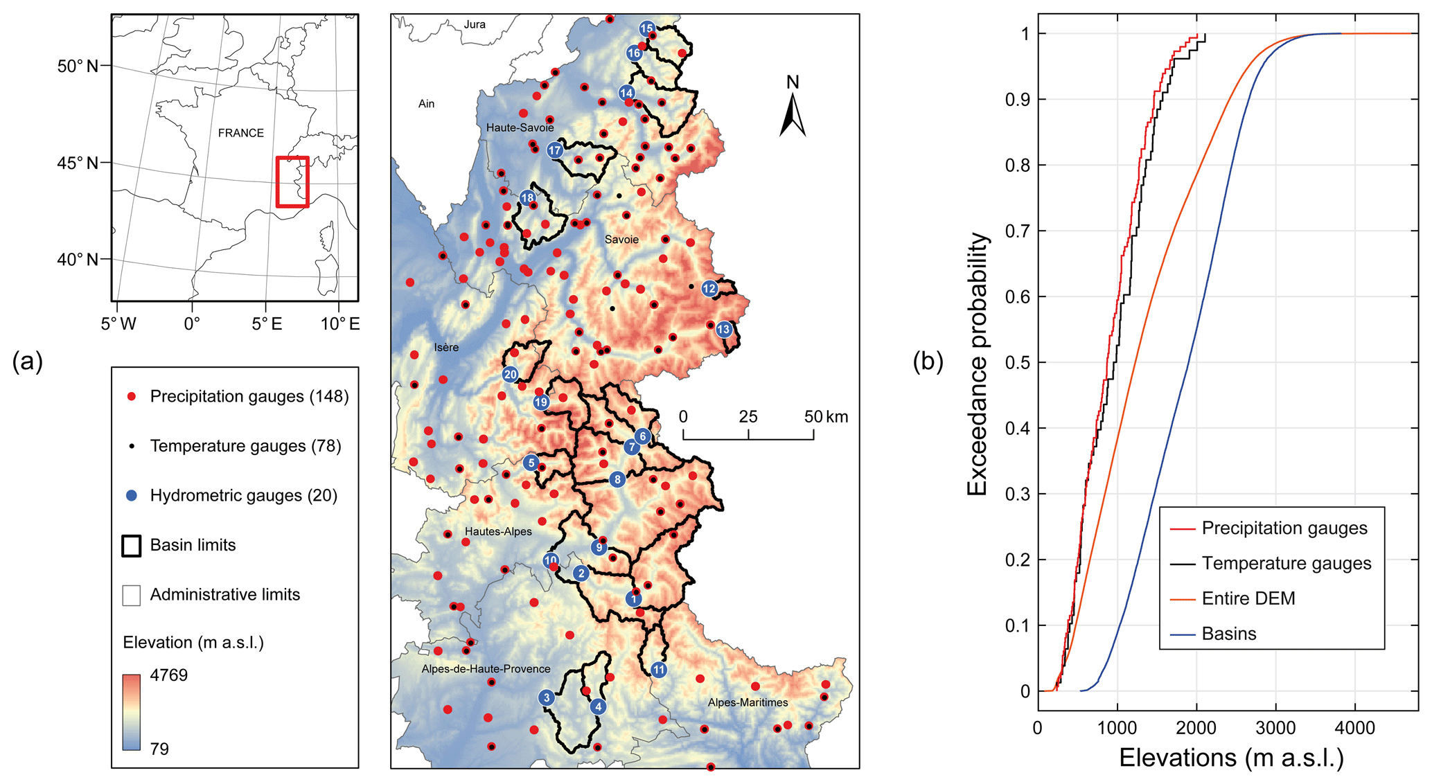
https://www.hydrol-earth-syst-sci.net/24/2609/2020/hess-24-2609-2020-f01

Figure 1Study area and data: (a) location of the selected precipitation, temperature, and streamflow stations, as well as elevations from a SRTM digital elevation model (DEM resampled to a grid with 0.5×0.5 km cells) in the French Alps; (b) elevation distributions of in situ stations, DEM, and basins. The station numbers refer to Table 1.

2.2 Streamflow data

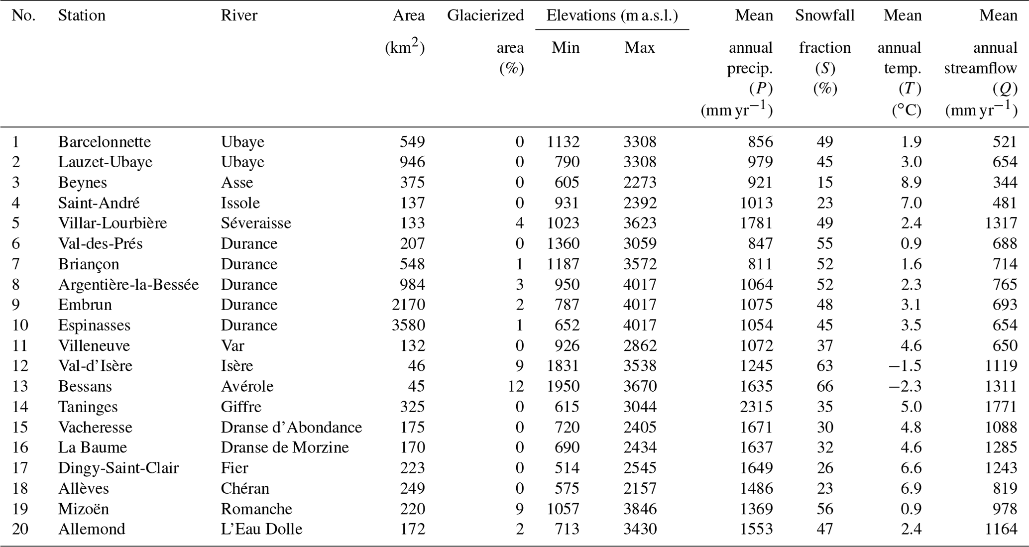
In order to avoid case-specific results, a dataset of 20 catchments was gathered from the French hydrological database (http://www.hydro.eaufrance.fr/, last access: May 2020) over the study area (Fig. 1 and Table 1). The catchments were selected based on the following criteria: (i) their streamflow regime is considered to be natural since they are located upstream from any major hydraulic installations, such as dams and water transfers; (ii) their streamflow regime is moderately to strongly affected by snow; and (iii) their streamflow series present good quality measurements according to the hydrological reports, with less than 10 % daily missing values for the period 2000–2016. The catchments are located on high reliefs (the median range of altitude is around 2000 m a.s.l.) and are differently affected by snow (between 15 % and 66 % of their total precipitation falls in the solid form). During the catchment selection process, we tried avoiding glacierized catchments to minimize possible interactions with non-snow-related processes that could also influence streamflow. Therefore, most catchments have zero or limited glacierized areas. Catchment areal precipitation and temperature were estimated after inferring altitudinal gradients, as detailed in the current paper. The dataset covers a large range of hydrological conditions, with mean annual precipitation, temperature, and streamflow ranging from 811 to 2315 mm, −2.3 to +8.9 ^∘C, and 344 to 1771 mm, respectively.

Table 1Streamflow gauging stations and main catchment characteristics. Percentages of glacierized area were estimated from the World Glacier Inventory (NSIDC, 2012). Mean annual precipitation (P), snowfall fraction (S), and temperature (T) were estimated after calibrating local altitudinal gradients over 2000–2016 using the snow-hydrological inverse approach proposed in the current paper (see Test no. 4 in Table 5).

Download Print Version | Download XLSX

2.3 Snow-cover data

MOD10A1 (Terra) and MYD10A1 (Aqua) snow products version 5 were downloaded from the National Snow and Ice Data Center for the period 24 February 2000–1 January 2017. This corresponds to 6157 dates, among which 98.8 % are available for MOD10A1 and 85.8 % for MYD10A1 since Aqua was launched in May 2002 and became operational in July 2002. These snow products are derived from a Normalised Difference Snow Index (NDSI) calculated from the near-infrared and green wavelengths and for which a threshold was defined for the detection of snow (Hall et al., 2006, 2007). Cloud cover represents a significant limit for these products, which are generated from instruments operating in the visible-near-infrared wavelengths. As a result, the grid cells were gap-filled to produce daily cloud-free snow cover maps of the study area. The different classes in the original products were first merged into three classes: no-snow (no snow or lake), snow (snow or lake ice), and no-data (clouds, missing data, no decision, or saturated detector). The missing values were then filled according to a gap-filling algorithm inspired by techniques proposed in the literature (Parajka and Blöschl, 2008; Gafurov and Bárdossy, 2009; Gascoin et al., 2015). The algorithm works in three sequential steps.

i.
Aqua–Terra combination: for every pixel, if no-data was found in MOD10A1, then the value from MYD10A1 was used instead. Priority was given to MOD10A1 because MYD10A1 was found to be less accurate (see Gafurov and Bárdossy, 2009).
ii.
Temporal deduction by sliding time filter: a no-data pixel was reclassified as snow (no-snow) if the same pixel was classified as snow (no-snow) in both the preceding and following grids. The preceding and following grids were searched within a sliding temporal window, whose size was incremented up to 9 d in order to reduce the remaining fraction of no-data pixels to below 10 % (Fig. 2a). It should be noted that three periods of gaps in an upper time window (11, 13, and 18 d) were present in the data because of technical failures of the MODIS sensor. In these cases, a longer time deduction was used beforehand to specifically fill these periods.
iii.
Spatial deduction based on elevation and neighbourhood filter: for each date and each pixel, a 3×3 neighbourhood spatial filter was used to account for the elevation and the data in the neighbouring pixels to fill the remaining no-data pixels. Two configurations were considered: either the central pixel has no-data and the algorithm tries to attribute a neighbouring value or the central pixel has a value that can be assigned to some of its neighbours. The two configurations were repeated until there were no more gaps (Fig. 2a).

The resulting database consists of 5844 binary (snow/no-snow) maps at 500 m spatial resolution for the period 2000–2016 (16 hydrological years, from 1 September 2000 to 31 August 2016). As a synthesis of these maps, snow-cover durations over the study area are presented in Fig. 2c.

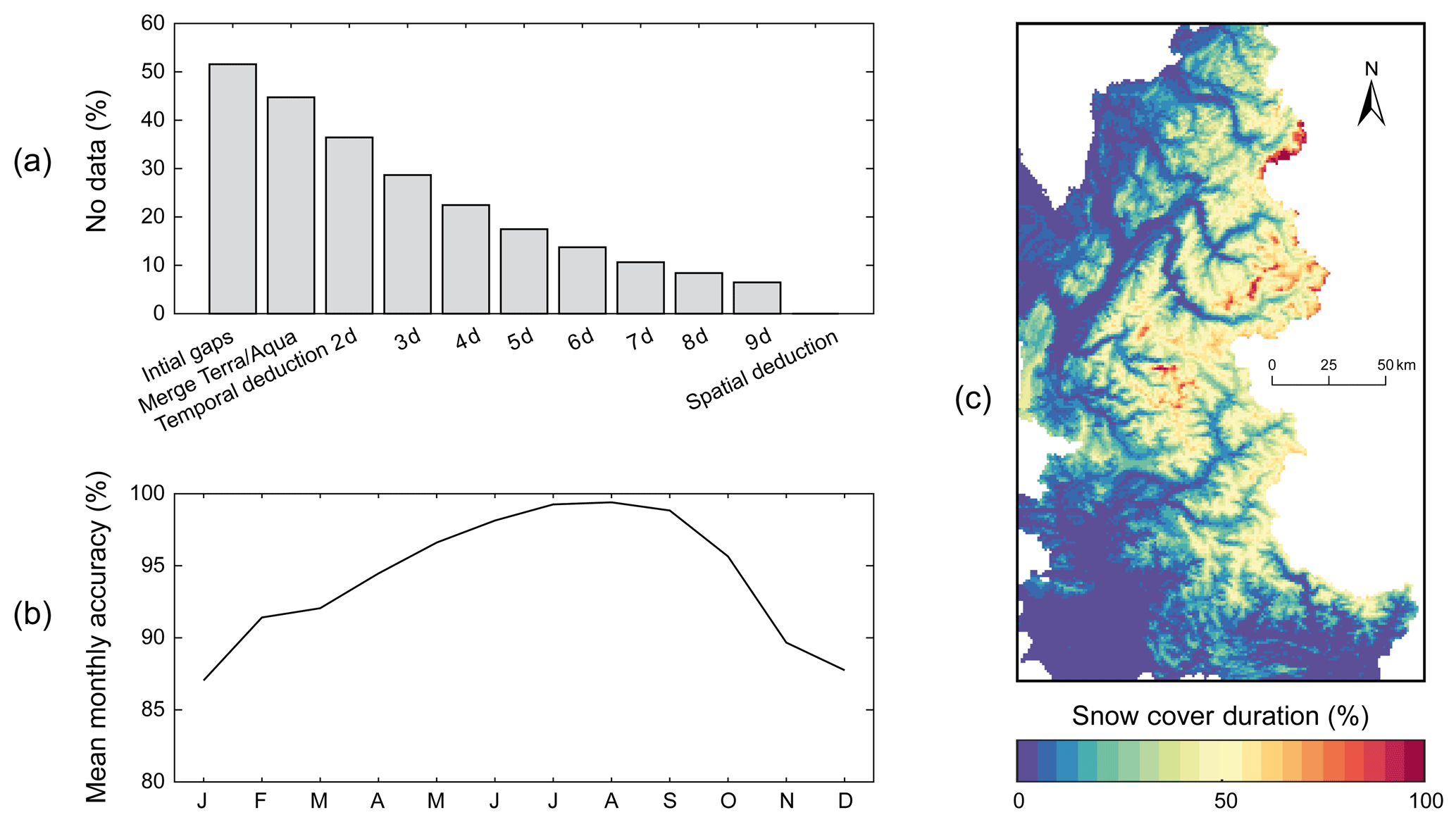
https://www.hydrol-earth-syst-sci.net/24/2609/2020/hess-24-2609-2020-f02

Figure 2Results of gap-filling applied to MODIS snow products: (a) evolution of the number of pixels classified as no-data (e.g. clouds) during the gap-filling procedure; (b) mean monthly accuracies according to validation based on confusion matrices with one image per month, i.e. ∼200 cloud-free images over the 2000–2016 period; (c) snow-cover duration based on gap-filled MODIS snow products over the 2000–2016 period.

In order to validate the gap-filling technique, a daily snow product with less than 10 % of no-data pixels was selected for each month of the studied period. These images were “blackened” (i.e. with 100 % no-data pixels) before applying the algorithm over the entire period to fill all gaps, including validation images. Filling accuracy was estimated for each image removed by computing confusion matrices which compared the pixels of the removed validation images and the filler reconstructions of these images. Validation based on confusion matrices with one image per month showed that the gap-filling technique applied to the MODIS snow products led to the reconstruction of images with average accuracies of 94 % (Fig. 2b). The mean monthly accuracies show greater ease in filling gaps in summer than in winter due to the differences in cloud obscuration. However, it should be noted that the actual accuracy of the MODIS gap-filling technique is necessarily greater than that of the validation procedure, in which many quality images needed to fill the gaps were missing.

3 Interpolation procedures

This section briefly presents the different spatial estimators used in the present study. The interpolation methods analysed include inverse distance weighted (IDW), ordinary kriging (ORK), kriging with external drift (KED), and IDW with external drift (IED). Interest readers can refer to Goovaerts (2000) for a detailed presentation of the different kriging algorithms and to Diggle and Ribeiro (2007) for their implementation in the public domain in the GeoPackage in R.

3.1 Spatial interpolation methods

3.1.1 Inverse distance weighting

Let us consider the problem of estimating the given variable z at an unsampled location u using only surrounding observation data. Let {z(u_α), α=1, …, n} be the set of data measured at n surrounding locations u_α. The inverse distance weighting (IDW) method estimated z as a linear combination of n(u) surrounding observations with the weights being inversely proportional to the square ω distance between observations and u:

\begin{matrix} (1) & \begin{aligned} Z_{IDW} (u) = & \frac{1}{\sum_{\propto = 1}^{n (u)} λ_{α} (u)} \sum_{\propto = 1}^{n (u)} λ_{α} (u) z (u_{α}), \\ with λ_{α} (u) = \frac{1}{{|u - u_{α}|}^{ω}} . \end{aligned} \end{matrix}

The basic idea behind the weighting scheme is that observations that are close to each other on the ground tend to be more alike than those located further apart; hence, observations closer to u should receive a larger weight.

3.1.2 Ordinary kriging

Instead of Euclidian distance, geostatistics uses the semivariogram as a measure of dissimilarity between observations. The experimental semivariogram is computed as half the average squared difference between the components of data pairs:

\begin{matrix} (2) & \hat{γ} (h) = \frac{1}{2 N (h)} \sum_{\propto = 1}^{N (h)} {[z (u_{α}) - (u_{α} + h)]}^{2}, \end{matrix}

where N(h) is the number of pairs of data locations a vector h apart. The hypotheses of spatial variability were here homogeneity and an isotropic spatial pattern due to the lack of sufficient sampled points, and hence identical variability in all directions.

Kriging is a generalized least-squares regression technique that makes it possible to account for the spatial dependence between observations, as revealed by the semivariogram, in spatial prediction. Like the inverse distance weighting method, ordinary kriging (ORK) estimates the unknown variable z at the unsampled location u as a linear combination of neighbouring observations:

\begin{matrix} (3) & Z_{ORK} (u) = \sum_{α = 1}^{n (u)} λ_{α}^{ORK} (u) z (u_{α}) with \sum_{α = 1}^{n (u)} λ_{α}^{ORK} (u) = 1 . \end{matrix}

The ordinary kriging weights $λ_{α}^{ORK} (u)$ are determined such as to minimize the estimation variance Var{Z_ORK(u)−z(u)} while ensuring the unbiasedness of the estimator $E {Z_{ORK} (u) - z (u)} = 0$ . These weights are obtained by solving a system of linear equations known as the ordinary kriging system:

\begin{matrix} (4) & \{\begin{cases} \sum_{β = 1}^{n (u)} λ_{β} (u) γ (u_{α} - u_{β}) - μ (u) = γ (u_{α} - u) & α = 1, \dots, n (u), \\ \sum_{β = 1}^{n (u)} λ_{β} (u) = 1, \end{cases} \end{matrix}

where μ(u) are Lagrange parameters accounting for the constraints on the weights. The only information required by the kriging system (Eq. 4) is semivariogram values for different lags, and these are readily derived once a semivariogram model has been fitted to experimental values. In this study, we dealt with the fitting of the semivariogram using two existing theoretical models, as presented below.

Exponential model
$\begin{matrix} (5) & γ (h; θ) \{\begin{array}{lc} 0, & h = 0, \\ θ_{0} + θ_{1} [1 - \exp (- 3 (∥h∥ / θ_{2}], & h \neq 0, \end{array} \end{matrix}$
for θ₀≥0, θ₁≥0 and θ₂≥0.
Spherical model
$\begin{matrix} (6) & γ (h; θ) \{\begin{cases} 0, & h = 0, \\ θ_{0} + θ_{1} (\frac{3 ∥h∥}{2 θ_{2}} - \frac{1}{2} {(\frac{∥h∥}{θ_{2}})}^{3}) & 0 < ∥h∥ \leq θ_{2}, \\ θ_{0} + θ_{1} & h > θ_{2}, \end{cases} \end{matrix}$
for θ₀≥0, θ₁≥0 and θ₂≥0.

The spherical model was tested because it is the most widely used semivariogram model and is characterized by linear behaviour (Goovaerts, 2000). The exponential model was selected in addition because it is recommended in the literature for spatial analysis of temperature (Tobin et al., 2011) and precipitation (Bárdossy and Pegram, 2013; Masson and Frei, 2014) in high-mountain regions. Each of these models was combined with a nugget effect, sill, and range as parameters. An automatic procedure was necessary to fit the semivariogram model to experimental values over the study period (1998–2016). The models were fitted using regression such that the weighted sum of squares of differences between the experimental and model semivariogram is minimum (see Goovaerts, 2000).

3.2 Accounting for elevation dependency

3.2.1 Kriging with external drift

Kriging with an external drift (KED) predicts sparse variables which are poorly correlated in space by considering that there is a local trend within the neighbourhood; primary data are assumed to have a linear relationship with auxiliary information exhaustively sampled over the study area (Ahmed and de Marsily, 1987). KED thus uses secondary information (such as elevation) to derive the local mean of the primary attribute z and then performs kriging on the corresponding residuals:

\begin{matrix} (7) & \begin{aligned} Z_{KED} (u) - m_{KED} (u) & = \sum_{α = 1}^{n (u)} λ_{α}^{KED} (u) [z (u_{α}) - m_{KED} (u_{α})], \\ with m_{KED} (u) = a_{0} (u) + a_{1} (u) y (u), \end{aligned} \end{matrix}

where y(u) are elevation data available at all estimation points, and a₀ and a₁ are two regression coefficients estimated from the set of collocated variables of interest and elevation data {z(u_α), y(u_α), α=1, …, n} using a simple linear relation.

The KED procedure was applied at each time step independently and within each search neighbourhood when the time series were interpolated. The coefficients a₀ and a₁ thus varied in space and time, which makes it possible to consider a variable space–time relationship between the primary variable (temperature or precipitation) and the secondary variable (elevation).

3.2.2 Inverse distance weighting with external drift (IED)

The external drift approach was also tested using the inverse distance weighting procedure to propose an original technique, which we called IDW with external drift (IED), as follows:

\begin{matrix} (8) & \begin{aligned} Z_{IED} (u) - m_{IED} (u) = & \frac{1}{\sum_{\propto = 1}^{n (u)} λ_{α} (u)} \sum_{\propto = 1}^{n (u)} λ_{α} (u) \\ [z (u_{α}) - m_{IED} (u_{α})], \\ with m_{IED} (u) = a_{0} (u) + a_{1} (u) y (u) . \end{aligned} \end{matrix}

3.3 Leave-one-out procedure

The interpolation parameters (n(u) and ω for IDW and IED, and n(u) and theoretical models for ORK and KED) were calibrated and the interpolation performance was assessed by “leave-one-out” cross-validation, which consists of the following principle: a successive estimation of all sampled locations was performed by using all other stations while always excluding the sample value at the location concerned. The spatial models were validated against RMSE (root mean square error) for temperature and precipitation at daily, monthly, and yearly timescales. Since the external drift computation and kriging weights can sometimes lead to negative precipitation amounts (Deutsch, 1996), a posteriori correction was performed to replace all negative-estimated precipitation values with a zero value.

The elevations of the gauging stations were used when applying the KED and IED procedures for the “leave-one-out” cross-validation. When interpolating temperature and precipitation exhaustively over the study area, the elevation predictors were based on the digital elevation model (DEM) of the Shuttle Radar Topography Mission (SRTM; Farr et al., 2007). The SRTM originally had a resolution of about 90 m. In this study, we used the SRTM elevation model resampled to a grid with 0.5×0.5 km cells from the UTM32N coordinate reference system. This spatial resolution was judged to be a good balance between computational constraints and elevation accuracy.

4 Model assessment methodology

The way of accounting for orographic gradients in the temperature and precipitation datasets was also assessed with respect to its ability to contribute to simulations of snow-covered area and streamflow at the catchment scale using the following modelling experiment.

4.1 Snow accounting routine (SAR)

The selected SAR (Fig. 3a) is a modified version of CEMANEIGE proposed by Valéry et al. (2014). The original version was modified to account for a snowfall under-catch correction factor as used in the HBV snow routine (see Beck et al., 2016), the computation of fractional snow-covered area (FSC) from a snow water equivalent (SWE) threshold, and possible integration of temperature and precipitation altitudinal gradients.

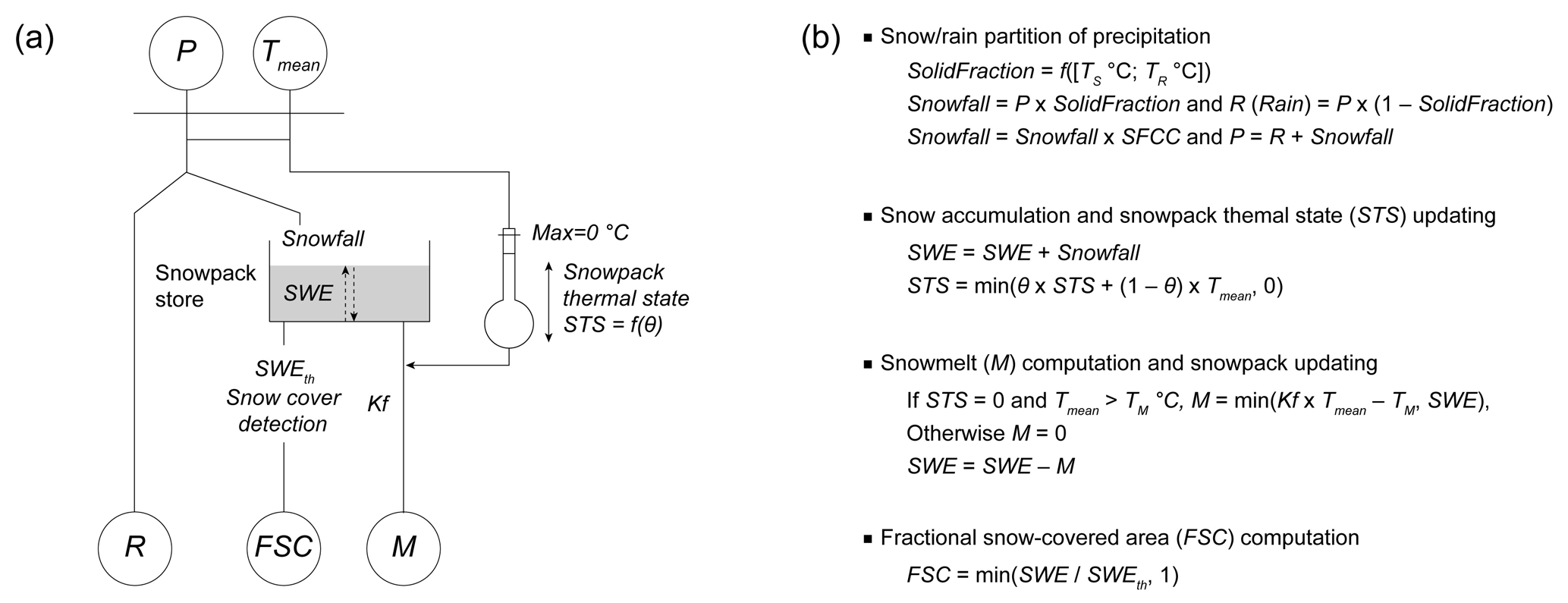
https://www.hydrol-earth-syst-sci.net/24/2609/2020/hess-24-2609-2020-f03

Figure 3Snow accounting routine: (a) conceptual scheme and (b) associated equations (modified from Valéry et al., 2014). P, R, T_mean, M, and FSC stand for total precipitation, rainfall, mean temperature, melt, and factional snow cover, respectively.

Download

Depending on the objectives, the model can be run in a full distributed mode or according to elevation bands. As distributed (or semi-distributed) inputs, it requires the daily liquid equivalent water depth of total precipitation (P) and mean daily air temperature (T_mean). In the case of a semi-distributed application at the catchment scale, the first step is to divide the catchment into elevation zones of equal area. Mean areal inputs (P and T_mean) are then extracted for each elevation zone from gridded temperature and precipitation datasets. In the present study, the number of elevation zones was set at five due to computational constraints and because preliminary tests showed no significant improvement in the snow-hydrological simulations when a higher spatial resolution (more elevation bands or full distribution) was used.

In each elevation band, the functions of the SAR described in Fig. 3b are applied with a unique set of parameters. Internal states (snowpack represented according to snow water equivalent (SWE) and its thermal state STS) vary independently in each elevation zone according to the differences in input values. When gridded temperature and precipitation datasets interpolated without elevation dependency are used, the SAR enables forcing data for each elevation zone to be modified based on two orographic gradients (TLR and PLR) used as key parameters:

\begin{matrix} (9) & \begin{aligned} T_{i} (t) & = T_{i}^{IDW} (t) + [\frac{(TLR + \frac{1}{2} TLR \times Si \times CSV)}{100} \\ \times (y_{i} - y_{i}^{IDW} (t))], \end{aligned} \end{matrix}

with:

\begin{matrix} (10) & \begin{aligned} Si \{\begin{cases} \sin (\frac{2 π \times (d - 80.5)}{366}), & lat > 0, \\ - s i n (\frac{2 π \times (d - 80.5)}{366}), & lat < 0, \end{cases} \\ P_{i} (t) = P_{i}^{IDW} (t) \times [1 + \frac{PLR}{1000} \times (y_{i} - y_{i}^{IDW} (t))], \end{aligned} \end{matrix}

where $T_{i}^{IDW} (t)$ and $P_{i}^{IDW} (t)$ are, respectively, the mean areal temperature and precipitation interpolated based on the IDW procedure in elevation zone i at time step t; $y_{i}^{IDW} (t)$ is the mean areal elevation interpolated based on the IDW procedure in elevation zone i from the available gauges at time step t; y_i is the mean areal elevation extracted from the DEM in elevation zone i; TLR and PLR are the constant temperature and precipitation lapse rates to be calibrated; CSV is a coefficient of seasonal variation due to solar radiation to be applied to TLR (when set to 0, no seasonal variation is applied); Si is an index of seasonal change in solar radiation accounting for daytime length and ranges from −1 on 21 December (winter solstice) to 1 on 21 June (summer solstice) in non-leap years in the Northern Hemisphere (lat > 0); d is the number of days since 1 January of the current year.

In the original version of CEMANEIGE, FSC area is calculated as follows:

\begin{matrix} (11) & {FSC}_{i} (t) = \min (\frac{{SWE}_{i} (t)}{{SWE}_{th}}, 1), \end{matrix}

where SWE is the quantity of snow accumulated in snow water equivalent (a state variable of the model, in mm), and SWE_th is the model's melting threshold. SWE_th is calculated as being equal to 90 % of mean annual solid precipitation on the catchment considered (Valéry et al., 2014). Alternative approaches have been proposed to account for the hysteresis that exists between FSC and SWE during the accumulation and melt phases (Riboust et al., 2019). However, introducing such a hysteresis adds two additional free parameters to the SAR. Instead, SWE_th was fixed to 40 mm since preliminary sensitivity analyses showed that this value gave satisfactory FSC values when compared to the MODIS observations in the studied catchments.

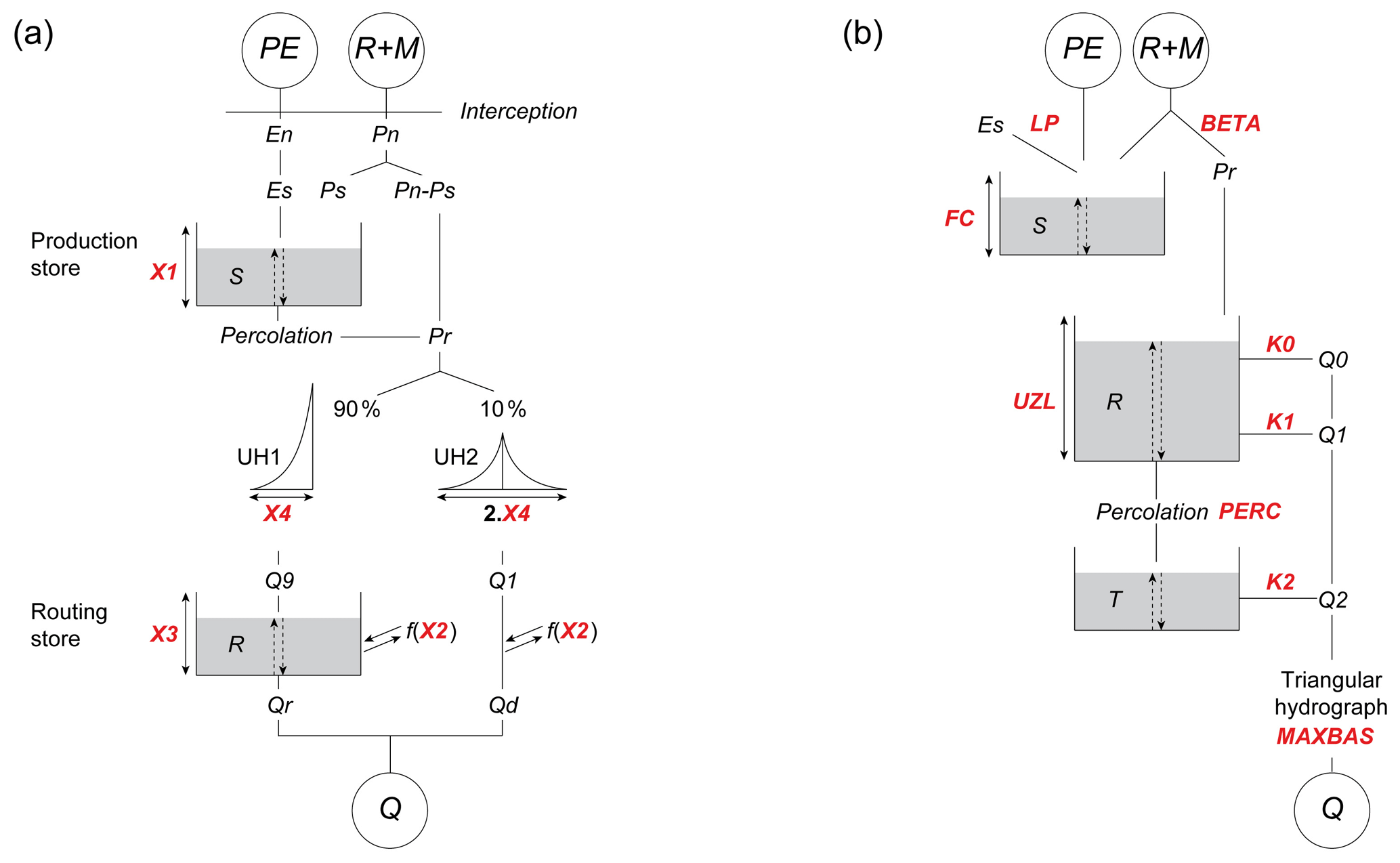
https://www.hydrol-earth-syst-sci.net/24/2609/2020/hess-24-2609-2020-f04

Figure 4Diagrams of the two hydrological models used: (a) GR4J and (b) HBV9. Calibrated parameters are in red and are further described in Table 3. R, M, PE, and Q stand for rainfall, snowmelt, potential evapotranspiration, and streamflow, respectively.

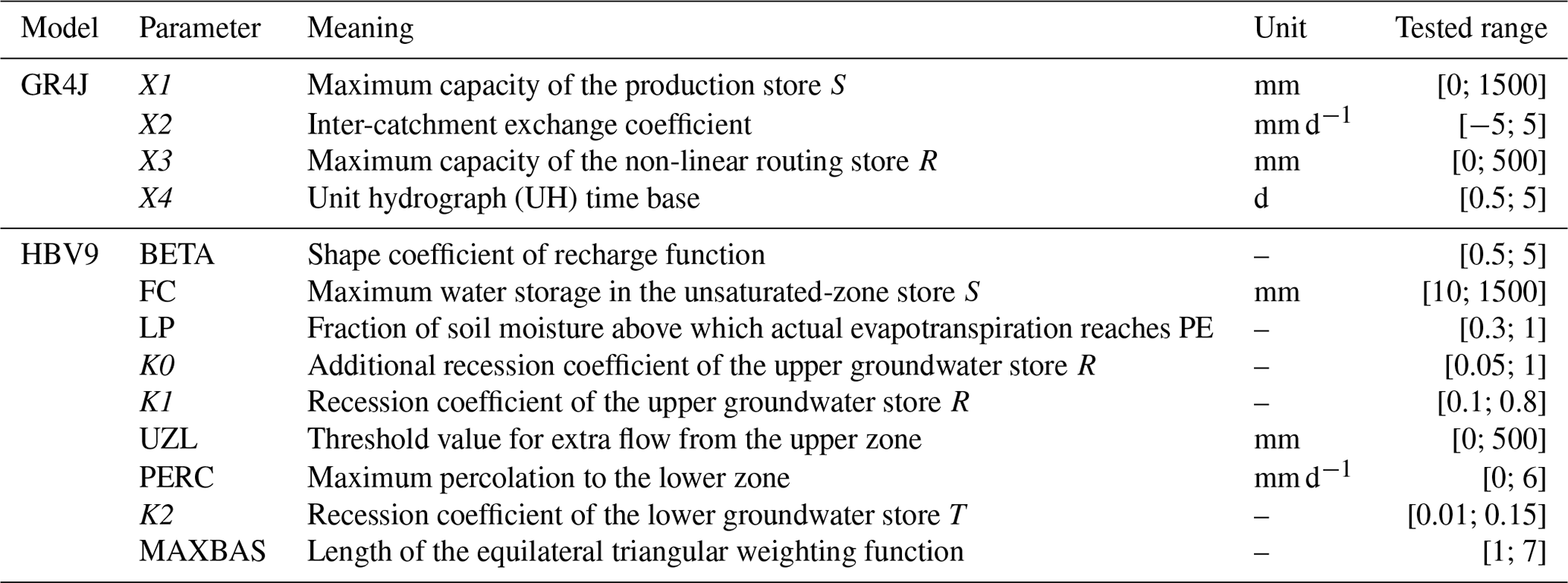
Table 2Parameters of the snow accounting routine and their associated fixed values or ranges tested in each modelling experiment.

Download Print Version | Download XLSX

To ensure insightful comparison with the modelling experiment, the SAR was calibrated according to different modes and degrees of freedom (Table 2). In mode M1, elevation dependency, which was accounted for (or not) in the T and P inputs based on the interpolation procedures, was tested by calibrating five parameters (T_S, T_R, SFCC, θ, Kf) which control snow accumulation and snowmelt. This mode is usually used to allow snow processes to be adjusted to local conditions and/or the errors in the T and P inputs. In mode M2, all parameters of the SAR were fixed in order to introduce two parameters (TLR and PLR) as orographic gradients. The aim of using this mode was to account for elevation dependency in the T and P inputs from constant, calibrated orographic gradients while fixing the parameters that control snow accumulation and snowmelt to physical or general values: precipitation phase determined based on a linear separation between −1 and +3 ^∘C (USACE, 1956), temperature threshold for snowmelt fixed at 0 ^∘C, and degree-day melt factor set at 5 mm ^∘C⁻¹ d⁻¹ (mean general value taken from Hock, 2003). In mode M3, the same approach was chosen, but an additional parameter (CSV) was associated with the TLR gradient in order to test the value of introducing a seasonal variation in the temperature lapse rates (see Eq. 9). In mode M4, elevation dependency in the T and P inputs was also accounted for based on three (TLR, CSV, and PLR) parameters, and two other parameters (θ, Kf) were calibrated in addition to allow for snowmelt adjustment.

In each altitudinal band, five outputs (rainfall, snowfall, snowmelt, potential evapotranspiration, and fractional snow-covered area) are computed at each daily time step. Rainfall (R) and snowmelt (M) are summed to compute the total quantity of water available for production and transfer in the catchment. Potential evapotranspiration (PE) is computed for each altitudinal band using the temperature-based formulation proposed by Oudin et al. (2005):

\begin{matrix} (12) & {PE}_{i} (t) = \frac{R_{e}}{λ ρ} \frac{T_{i} (t) + 5}{100} if (T_{i} (t) + 5) >; else {PE}_{i} (t) = 0, \end{matrix}

where R_e is the extra-terrestrial solar radiation (MJ m⁻² d⁻¹) which depends on the latitude of the basin and the Julian day of the year, λ is the net latent heat flux (fixed at 2.45 MJ kg⁻¹), ρ is the water density (set at 11.6 kg m⁻³), and T_i(t) is the air temperature (^∘C) estimated in the elevation zone i at time step t.

The outputs of each band are averaged to estimate the total liquid output of the SAR and PE at the catchment scale in order to feed the combined hydrological models (Fig. 4).

Table 3Parameters of the hydrological models and their associated ranges tested.

Download Print Version | Download XLSX

4.2 Hydrological models

To avoid model-specific results, two well-known hydrological models (see structures in Fig. 4 and parameters in Table 3) were chosen in association with the SAR: the four-parameter GR4J presented by Perrin et al. (2003) and a nine-parameter lumped version of the HBV model (Bergström, 1975; Beck et al., 2016), here referred to as HBV9 to avoid confusion with the original version.

The two models were run at a daily time step and used in lumped mode with the SAR on top. The structure and the number of degrees of freedom differ between GR4J and HBV9, which should make results more generalizable.

4.3 Calibration and validation methods

4.3.1 General model assessment

The models (GR4J and HB9 with the SAR on top) were cross-validated using a split-sample test procedure. The simulation period (2000–2016) was split into two sub-periods alternatively used for calibration and validation. Thus two calibration and two validation tests were performed to provide evaluation on all available data. Mean annual precipitation increased by around 17 % between the two periods, while mean annual temperature was stable (9.2 ^∘C vs. 9.3 ^∘C) across the in situ network presented in Sect. 2.1. Although the second period was generally wetter, differences can be observed locally. At the basin scale, the differences between the two periods ranged from −10 % to +15 % for precipitation, −0.5 to +0.5 ^∘C for temperature, and −11 to +50 % for streamflow.

The models were run in a continuous way for the whole reference period, while only hydrological years (from 1 September to 31 August) corresponding to the calibration and validation periods were considered to compute the efficiency criteria. The 3-year period before the simulation period was used for model warm-up to limit the effect of the storage initialization and was not included in performance computation.

4.3.2 Optimization algorithm and objective function

The parameters of the SAR and the hydrological model were optimized simultaneously, using the shuffled complex evolution (SCE) algorithm (Duan et al., 1992). The algorithmic parameters of SCE were set to the values recommended by Duan et al. (1994) and Kuczera (1997) to reduce the risk that SCE fails in local optimal solutions. The objective function (OF) used was a multi-criteria composite function focusing simultaneously on variations in snow-covered areas and streamflow dynamics at the basin scale, as follows:

OF = 1 - (0.5 \times {NSE}_{SNOW} + 0.5 \times {NSE}_{sqr Q}),

with

\begin{matrix} (13) & {NSE}_{SNOW} = \frac{1}{E} \sum_{i = 1}^{E} (1 - \frac{\sum_{t = 1}^{N} {({FSC}_{sim, t}^{i} - {FSC}_{obs, t}^{i})}^{2}}{\sum_{t = 1}^{N} {({FSC}_{obs, t}^{i} - {\overline{FSC}}_{obs}^{i})}^{2}}), \end{matrix}

{NSE}_{sqr Q} = 1 - \frac{\sum_{t = 1}^{N} {(\sqrt{Q_{sim, t}} - \sqrt{Q_{obs, t}})}^{2}}{\sum_{t = 1}^{N} {(\sqrt{Q_{obs, t}} - \sqrt{\overline{Q_{obs}}})}^{2}},

where FSC $_{obs, t}^{i}$ and FSC $_{sim, t}^{i}$ are the observed and simulated FSC areas in elevation zone i at daily time step t, N is the total number of time steps, ${\overline{FSC}}_{obs}^{i}$ is the mean observed FSC in elevation zone i over the test period, E is the total number of elevation zones (fixed to five for the study), Q_obs,t and Q_sim,t are the observed and simulated streamflows at daily time step t, and $\sqrt{\overline{Q_{obs}}}$ is the mean observed square root transformed flows over the test period.

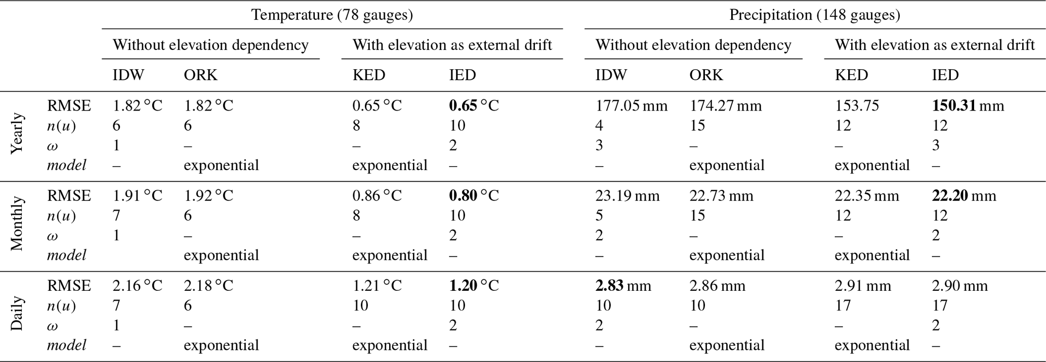
Table 4Cross-validation of the interpolation methods against yearly, monthly, and daily series from meteorological gauges over the period 2000–2016. The best efficiency criteria for each analytical timescale and each variable of interest (temperature and precipitation) are in bold. The values of n(u) and ω (for IDW and IED) and of n(u) and model (for ORK and KED) represent the interpolation parameters, which were optimized using the leave-one-out procedure, as described in Sect. 3.3.

Download Print Version | Download XLSX

NSE_SNOW relies on the Nash–Sutcliffe efficiency criterion. Perfect agreement between the observed and simulated values gives a score of 1, whereas a negative score represents lower reproduction quality than if the simulated values had been replaced by the mean observed values. NSE_sqrQ can be considered a multi-purpose criterion focusing on the simulated hydrograph. It puts less weight on high flows than the standard NSE on non-transformed discharge (Oudin et al., 2006). As the majority of basins had negligible glacierized areas (see Table 1), no specific glacier model was activated. This led to neglect of the late summer contribution of glacier melt to river discharge in the three basins with 9 %–12 % glacierized areas.

4.3.3 Efficiency criteria in validation

Four criteria were used to evaluate model performance during validation. The first one was the NSE_SNOW criterion. To put more emphasis on high- and low-flow conditions, we used the NSE on non-transformed streamflows (NSE_Q), which gives more weight to large errors generally associated with peak flows, and the NSE on log-transformed streamflows (NSE_ln Q). The absolute cumulated volume error (VE_C) was also computed to obtain information on the agreement between observed and simulated total discharge over the test periods:

\begin{matrix} (14) & {VE}_{C} = 1 - \frac{|\sum_{t = 1}^{N} Q_{sim, t} - \sum_{i = 1}^{N} Q_{obs, t}|}{\sum_{t = 1}^{N} Q_{obs, t}} . \end{matrix}

A value of 1 indicates perfect agreement, while values less than 1 indicate over- or under-estimation of the volume.

5 Results and discussion

5.1 Cross-validation of the interpolation methods

Table 4 lists the results of cross-validation of the interpolation methods against yearly, monthly, and daily series from temperature and precipitation gauges. Kriging with ORK led to an improvement over IDW only for precipitation interpolation at the yearly and monthly timescales. Considering elevation dependency with external drift (KED and IED) improved the performance of the kriging and inverse-distance methods, except for precipitation estimated at the daily timescale. This shows that the correlation between precipitation and topography increases with the increasing time aggregation as already reported in other studies (e.g. Bárdossy and Pegram, 2013; Berndt and Haberlandt, 2018). The elevation dependency of precipitation thus depends significantly on the accumulation time. At the daily timescale, the orographic enhancement is limited because on a given day there is no monotonic relationship between elevation and precipitation amount: it depends on where the precipitation event occurs in the first place.

Of all the methods tested, IED provided the best performance in terms of lower RMSE for each variable (temperature and precipitation) and at all temporal resolutions (yearly, monthly, and daily), except for precipitation at the daily timescale for which IDW performed best.

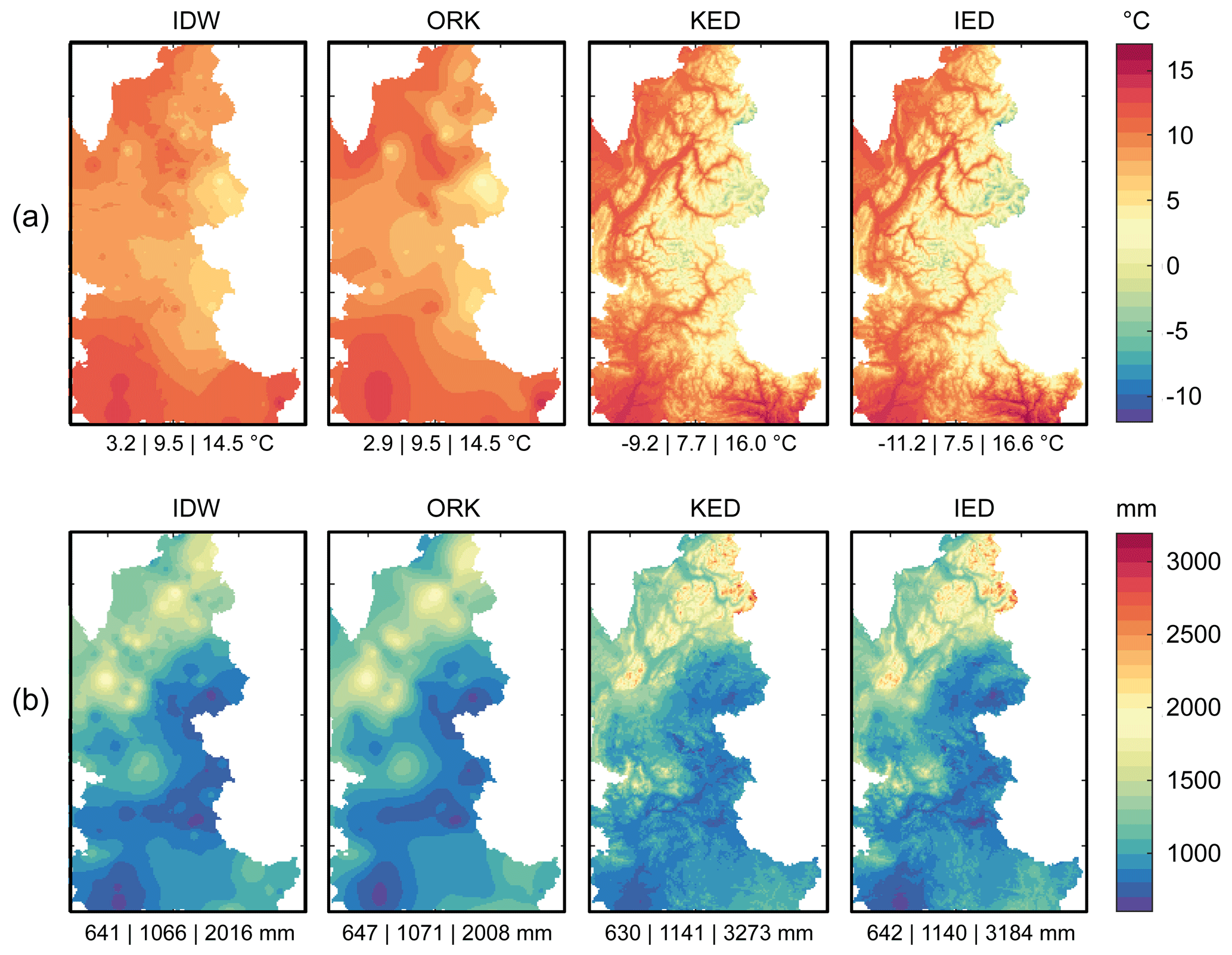
https://www.hydrol-earth-syst-sci.net/24/2609/2020/hess-24-2609-2020-f05

Figure 5Maps of mean annual temperature (^∘C) and total precipitation (mm yr⁻¹) obtained by interpolation of (a) 78 gauges (temperature) and of (b) 148 gauges (precipitation) with daily data for the period 2000–2016 using inverse distance weighting (IDW), ordinary kriging (ORK), kriging with external drift (KED), and IDW with external drift (IED). The numbers below each map stand, respectively, for minimum, mean, and maximum values (expressed in ^∘C for temperature and in mm yr⁻¹ for precipitation) in the maps.

Download

The exponential variogram model for the ORK and KED method performed systematically better than the spherical model whatever the variable and the timescale. In contrast, the exponent ω used with the IDW and IED methods varies from 1 to 3 depending on the considered variable and timescale. The optimized number of surrounding neighbours n(u) also varies depending on the method and timescale. At the daily timescale, n(u) ranged from 6 when interpolating temperature with ORK to 17 when interpolating precipitation with KED and IED. Hence, 10 (17) surrounding neighbours were used to compute altitudinal gradients of temperature (precipitation) based on the daily linear regressions with KED and IED.

Figure 5 shows the annual temperature and precipitation maps obtained by interpolating daily data from the meteorological gauges over the period 2000–2016 using the IDW, ORK, KED, and IED methods and their optimized parameters (Table 4). The maps of IED estimates of mean temperature and annual precipitation closely resemble the KED maps. Temperature estimates range from −9.2 to 16.0 ^∘C with KED and from −11.2 to 16.6 ^∘C with IED. Precipitation estimates range from 630 to 3273 mm with KED and from 642 to 3184 mm with IED. As expected, these ranges are wider than those obtained with the IDW and ORK procedures, which, unlike the KED and IED methods, do not consider either local or seasonal elevation dependency. As a result, the ranges obtained with KED and IED are probably more realistic with respect to temperature, but not necessarily with respect to precipitation, for which daily cross-validation shows that the simple IDW method provided better results. However, cross-validation was based on gauges sampled only below 2006 (2105) m a.s.l., meaning evaluation of the precipitation (temperature) gridded datasets at higher altitudes was not possible. Another approach is thus needed to further explore whether elevation dependency should be disregarded when estimating daily precipitation (as suggested by cross-validation), and, if not, whether this dependency should be accounted for in the interpolation process or by inverting the hydrological cycle. A sensitivity analysis of snow-hydrological simulations to the orographic gradients was thus conducted.

5.2 Sensitivity of the snow-hydrological simulations to the orographic gradients

For the sake of brevity, here we only present the results obtained with the datasets interpolated with the IDW and IED procedures, since cross-validation at the daily timescale showed that they slightly outperformed the ORK and KED methods, respectively. Table 5 summarizes the six tests performed to account for elevation dependency in the T and P inputs via the modelling experiment described in Sect. 4.

Table 5Description of the tests to account for elevation dependency in the T and P inputs via the modelling experiment described in Sect. 4. Note that each calibration test also included the hydrological parameters of GR4J or HBV9 (the parameter ranges tested are listed in Table 2 for the SAR and in Table 3 for the hydrological models).

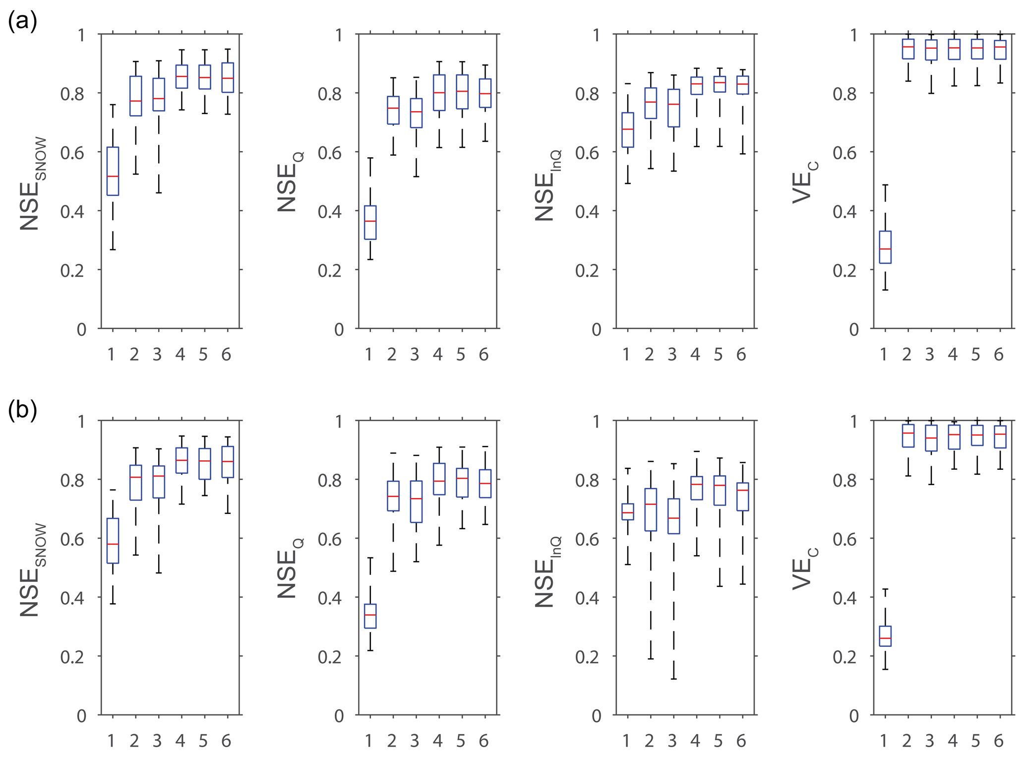
Download Print Version | Download XLSX

https://www.hydrol-earth-syst-sci.net/24/2609/2020/hess-24-2609-2020-f06

Figure 6Boxplots (showing 0.00, 0.25, 0.50, 0.75, and 1.00 percentiles) of the efficiency distributions obtained in validation by the (a) GR4J and (b) HBV9 models combined with the snow model according to six different tests (see Table 5) to account for elevation dependency in the T and P inputs on the 20 snow-affected Alpine catchments.

Download

Table 6Mean validation efficiency of the six modelling tests (see Table 5) on the set of 20 catchments with the GR4J model and the HBV9 model.

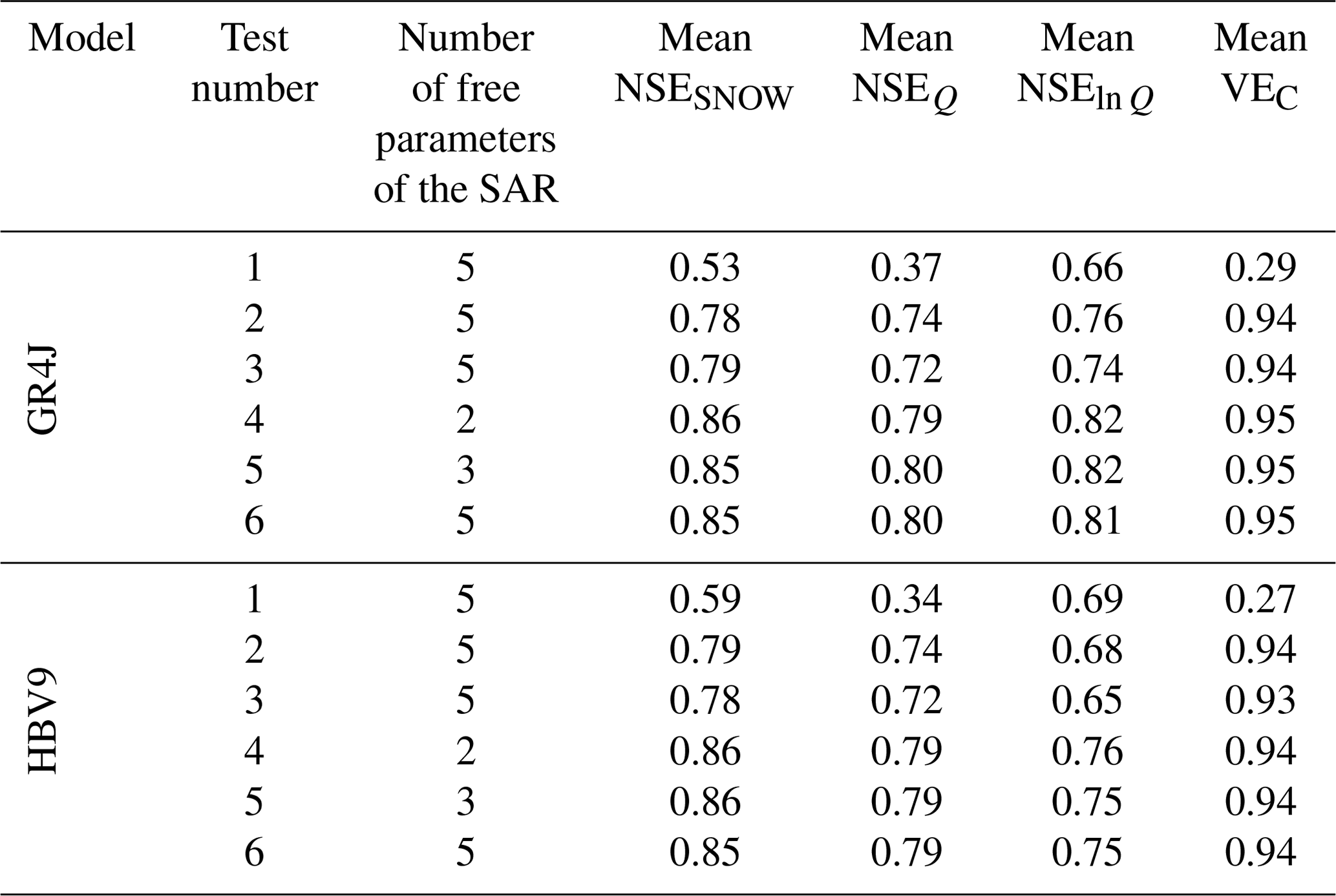
Download Print Version | Download XLSX

Figure 6 and Table 6 summarize the efficiency distributions obtained in validation with the GR4J and HBV9 models combined with the snow model in the different tests on the 20 snow-affected Alpine catchments. The results produced by the two hydrological models are in agreement and highlight the following main findings.

Not considering elevation dependency in either the T or P inputs (Test no. 1) leads to notable failures of the snow-hydrological models, due to incorrect snow–rainfall partitioning and snowmelt in space and over time caused by too high temperatures and insufficient input volumes of precipitation, which cannot be offset by the free parameters of the SAR. Notably, calibrating temperature thresholds and ranges for snow–rain partition and snowmelt, as well as snow under-catch (using the SFCC parameter), is clearly unsatisfactory.
Considering elevation dependency only in the T inputs based on the IED procedure (Test no. 2) significantly improves the snow-hydrological simulations, but considering elevation dependency in the P inputs based on the same procedure (Test no. 3) is not as efficient, notably for streamflow simulations. This shows that the estimated precipitation with IED over the catchments is of limited accuracy.
Improving the areal temperature and precipitation estimation clearly requires the calibration of altitudinal temperature and precipitation gradients. The snow-hydrological simulations are considerably improved when using the parsimonious two-parameter SAR based only on the calibration of TLR and PLR (Test no. 4).
Compared to Test no. 4 based only on a two-parameter SAR, only limited improvements in the performance distributions are obtained by introducing additional free parameters to account for the seasonal variability of the temperature gradients (Test no. 5) and for local adjustment of snowmelt (Test no. 6).

As a representative example of the studied catchments, Fig. 7 illustrates the differences in the simulations obtained by Test nos. 1 to 4 for the Durance at Serre-Ponçon. This 3580 km² catchment with altitudes ranging between 652 and 4017 m a.s.l. ensures inflows to one of the biggest dams in Europe (maximum capacity of 1.3 km³). Dynamics of fractional snow-cover area and streamflow are better simulated when considering elevation dependency of the T and P inputs via two calibrated, altitudinal gradients (Test no. 4). Compared to the other tests, mean annual temperature (4.0 ^∘C) is lower and mean annual precipitation (1160 mm) is higher. Less precipitation is considered in solid form (44 % of total precipitation on average) and accumulation is longer during winter, which fits streamflow observations better, both for low flows from December to April and for flood peaks between May and July. It is worth noting that these improved simulations were obtained with a SAR calibrated on only two parameters targeting the local lapse rates, whereas the other simulations were based on a SAR calibrated on five parameters. This shows that calibrating the usual snow parameters to compensate for errors in the input data and/or to adapt to local snow-related processes is less efficient in the simulations than inferring only temperature and precipitation lapse rates while fixing all the other parameters. This suggests that correcting for temperature and precipitation distribution has a stronger impact on model predictions than adjusting for snow-related processes like phase partitioning or melt and that correctly estimating total accumulation is likely to play a first-order role in the snow-hydrological responses of the studied catchments.

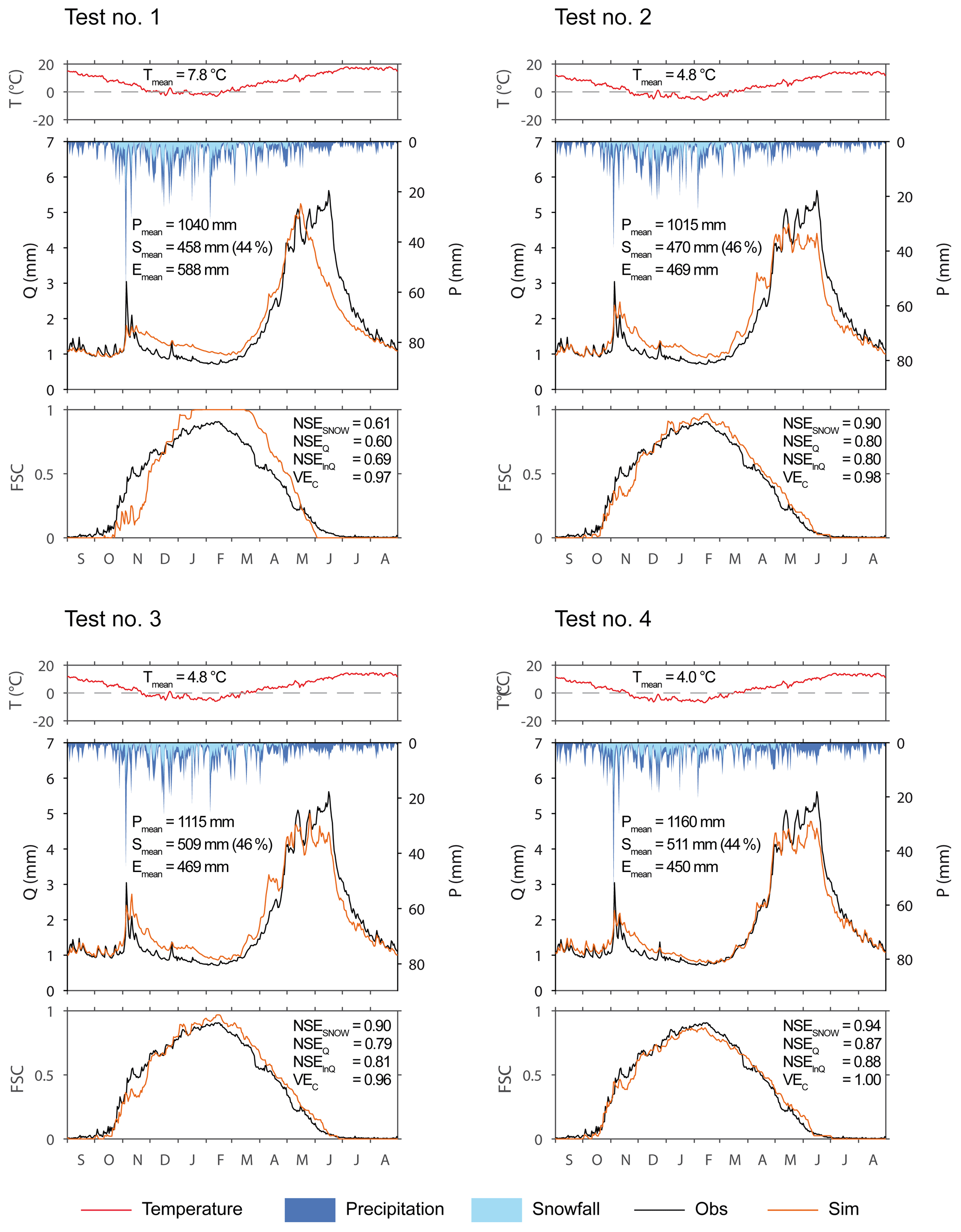
https://www.hydrol-earth-syst-sci.net/24/2609/2020/hess-24-2609-2020-f07

Figure 7Comparison of snow-hydrological simulations with elevation dependency according to Test nos. 1 to 4 (see Table 5) with GR4J for the Durance at Serre-Ponçon. The graphs show mean inter-annual time series of temperature, precipitation, streamflow, and fractional snow cover at the catchment scale in validation over the period 2008–2016. T_mean, P_mean, and S_mean stand for mean annual temperature, precipitation, and snowfall, respectively. The efficiency criteria NSE_SNOW, NSE_Q, NSE_ln Q, and VE_C are computed from continuous (not mean seasonal) series over 2008–2016.

Download

5.3 Identifiability of the parameters

Figure 8 shows a representative example of parameter sensitivity to the objective function (OF) according to the six tests (see Table 5) with the GR4J model on the Durance at Serre-Ponçon. The maximum allowed parameter range is only reached for the parameters X1 and X2 with Test no. 1. This test differs from the others because no elevation dependencies in the T and P inputs are considered. Consequently, hydrologic predictions of Test no. 1 are significantly outperformed by the other approaches. Extending the parameter ranges beyond the tested values would be both poorly efficient in improving the simulations and incorrect from a numerical point of view since they were set to values recommended by the models' authors. Moreover, no maximum parameter limits were reached in the other tests, thus suggesting that the parameter ranges are adequate.

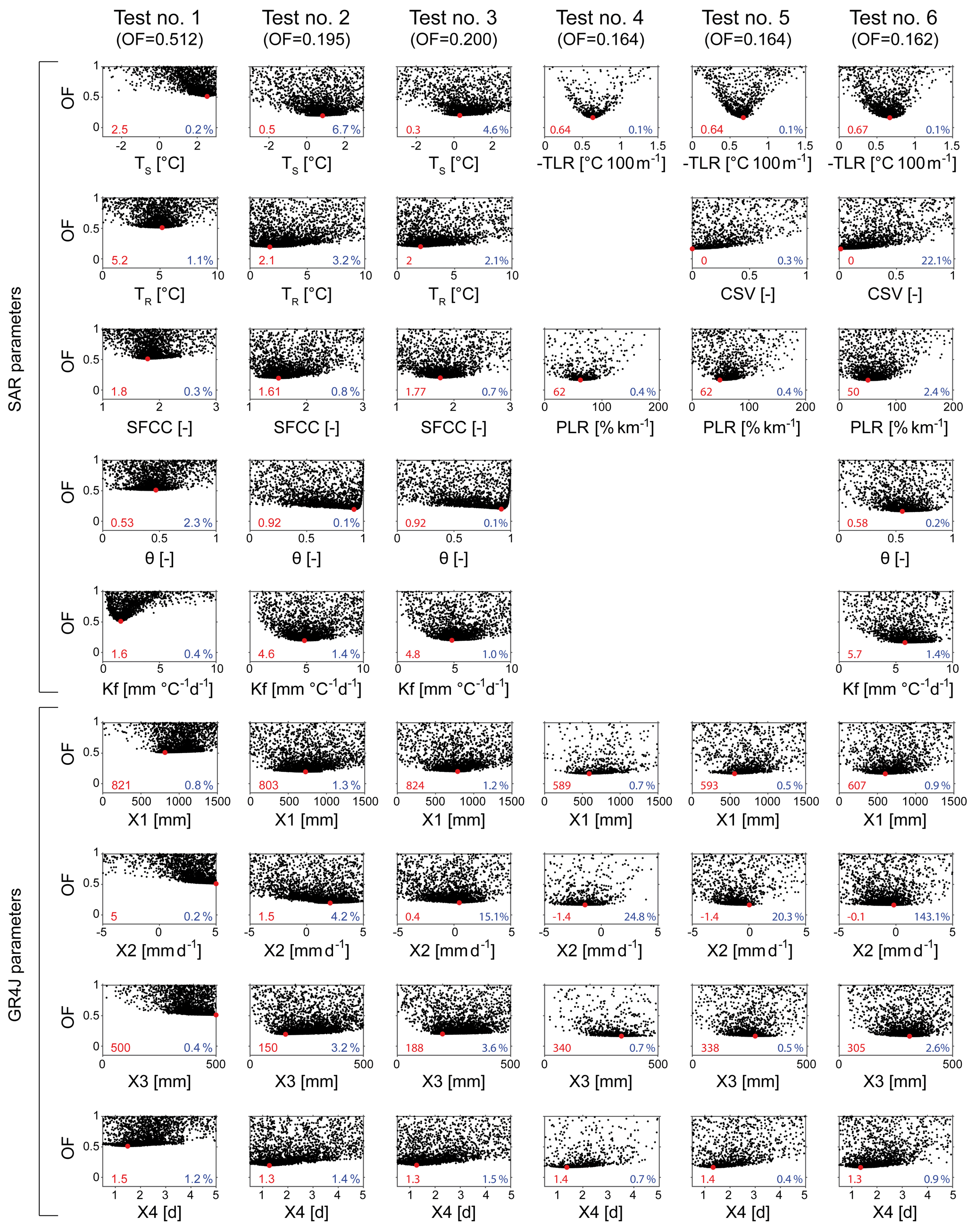
https://www.hydrol-earth-syst-sci.net/24/2609/2020/hess-24-2609-2020-f08

Figure 8Parameter sensitivity to the objective function (OF) according to Test nos. 1 to 6 (see Table 5) with GR4J combined with the snow accounting routine (SAR) on the Durance at Serre-Ponçon. The values and dots in red indicate the optimized calibrated parameters when minimizing OF, the black dots represent trials of the SCE-UA optimization algorithm, and the values in blue are the variation coefficients (in %) of the 20 % best-performing parameter solutions compared to the optimized values for each parameter (the lowest value, the easiest parameter identifiability). Note that, depending on the tests, the calibrated parameters of the SAR vary from 2 to 5 (see Tables 2 and 5), while the GR4J hydrological model has four free parameters (see Table 3).

Download

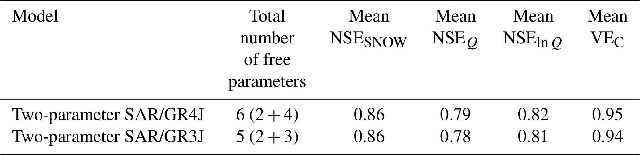
Table 7Mean validation efficiency on the set of 20 catchments with the GR4J model and the GR3J model in association with the two-parameter SAR.

Download Print Version | Download XLSX

As already shown, considering elevation gradients (Test nos. 4–6) minimizes OF and significantly improves model performance. It also improves the parameter identifiability. The temperature altitudinal gradient (TLR) is easily identifiable, with values ranging from −0.64 ^∘C per 100 m (Test nos. 4 and 5) to −0.67 ^∘C per 100 m (Test no. 6) and with variation coefficients of 0.1 % for the 20 % best-performing parameter solutions. It clearly proves to be a key parameter for improving snow and streamflow simulations compared to parameters calibrated using elevation gradients inferred from the usual interpolation method with external drift (Test nos. 2 and 3). The optimum value of the CSV parameter (Test nos. 5 and 6) is zero, clearly indicating no need to account for the seasonal variation in the temperature lapse rate in the catchment studied here (which is also the case in most catchments). The precipitation lapse rate (PLR) is also easy to identify, with optimized values of 62 % km⁻¹ (Test nos. 4 and 5) and variation coefficients 0.4 %. Introducing additional parameters controlling snowmelt (θ and Kf in Test no. 6) does not significantly improve the simulations and decreases the parameter identifiability (variation coefficients increase compared to Test nos. 4 and 5 based on a two-parameter and three-parameter SAR, respectively). This shows that model performance is mainly sensitive to the use of parameters for temperature and precipitation lapse rates and that a two-parameter SAR based on TLR and PLR (Test no. 4) on top of the hydrological models tested is both essential and sufficient to achieve satisfactory simulations.

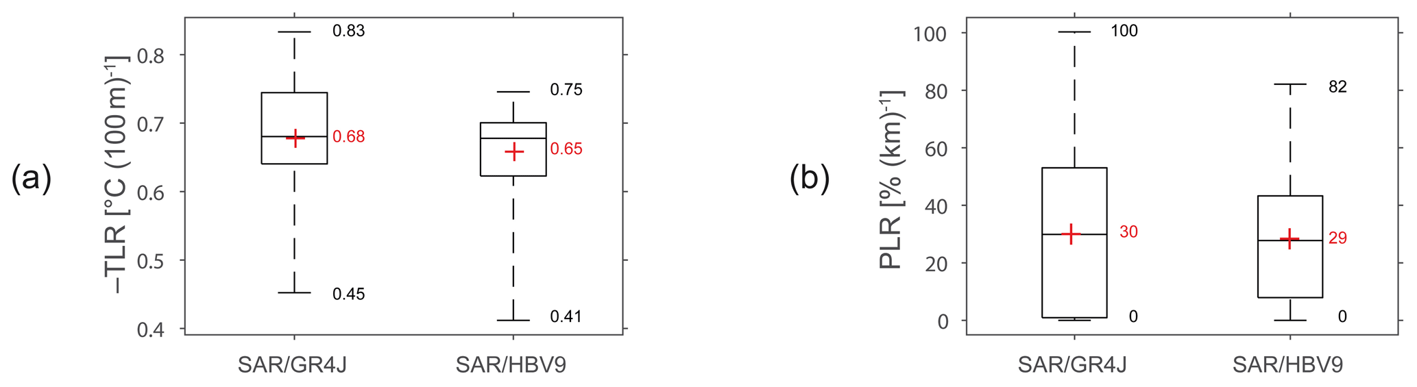
https://www.hydrol-earth-syst-sci.net/24/2609/2020/hess-24-2609-2020-f09

Figure 9Boxplots (showing 0.00, 0.25, 0.50, 0.75, and 1.00 percentiles) of the ranges of (a) temperature and (b) precipitation lapse rates calibrated with the two-parameter SAR (Test no. 4) in association with the GR4J and HBV9 models on the 20 snow-affected Alpine catchments. The red crosses indicate mean values.

Download

Equifinality is also reduced in Test nos. 4–6 for the parameters controlling runoff generation and routing (X1, X3, and X4). On the opposite end, the parameter of the inter-catchment groundwater flows (X2) is poorly identifiable, with variation coefficients of 24.8 %, 20.3 %, and 143.1 % with Test no. 4, Test no. 5, and Test no. 6, respectively. This suggests that inter-catchment groundwater exchanges (IGE) do not play a key role in the studied catchments. Indeed, fixing X2 to a value of 0 (i.e. without potential IGE) with an alternative GR3J model provided similar mean validation efficiency on the set of catchments as compared to the GR4J associated with the two-parameter SAR (Table 7). However, other objective functions may result in other findings as far as IGE are concerned. For instance, additional tests (not shown here for the sake of brevity) confirmed that it was possible to greatly reduce the X2 equifinality without decreasing the model efficiency by adding a water balance term in the objective function to constrain the proportion of years respecting the water and energy balance in the Turc–Budyko non-dimensional graph (see Andréassian and Perrin, 2012). These tests suggested that it may be relevant to explicitly represent inter-catchment groundwater transfers in association with correcting or scaling factors applied to the precipitation input data to render the distribution between evapotranspiration, streamflow, and underground fluxes more realistic, as already reported by Le Moine et al. (2007).

5.4 Ranges of the calibrated altitudinal gradients

Figure 9 shows that the temperature and precipitation lapse rates vary considerably from one catchment to another.

The mean values of the calibrated temperature lapse rates are −0.68 and −0.65 ^∘C (100 m)⁻¹ with GR4J and HBV9, respectively. These values are higher than the yearly lapse rates identified by Rolland (2003) from gauge observations in Alpine regions, which ranged from −0.54 to −0.58 ^∘C (100 m)⁻¹ in the Italian and Austrian Tyrol. Instead, the mean calibrated values are close to the average temperature gradients generally proposed as approximations in the literature (−0.65 ^∘C (100 m)⁻¹ in Barry and Chorley, 2010). They can be used as suitable estimates for daily snow-hydrological purposes in the French Alps. However, to better account for local meteorological conditions, it may be advisable to calibrate them since the TLR parameter ranges from −0.41 to −0.83 ^∘C (100 m)⁻¹, depending on the catchments and on the models, and is easily identifiable (see Fig. 8 and Sect. 5.3.).

The mean value of the calibrated precipitation lapse rates is 30 % (km)⁻¹ and 29 % (km)⁻¹ with GR4J and HBV9, respectively. The differences in ranges between the two models may be due to the GR4J ability to gain (or lose) water from inter-catchment groundwater flows through its X2 parameter (see Sect. 5.3), unlike HBV9, which considers the catchment to be a closed system. On the other hand, HBV9 relies on more parameters for production and transfer, thus enabling one to compensate differently for the errors in the precipitation volumes. Whatever the model, the calibrated lapse rates indicate the need for increased precipitation volumes in most catchments, either to counterbalance for erroneous measurements such as the systematic errors associated with precipitation under-catch during snowfall or to consider the orographic effect that cannot be sufficiently accounted for by the gauges used for interpolating the precipitation fields. However, the ranges of the precipitation lapse rates, from 0 % (km)⁻¹ to 100 % (km)⁻¹ with GR4J and from 0 % (km)⁻¹ to 82 % (km)⁻¹ with HBV9, suggest that the required correction is catchment-specific and depends either on the local meteorological conditions or on data from the available surrounding stations to interpolate the daily precipitation.

6 Summary and conclusions

6.1 Synthesis

In this paper, several alternative approaches for distributing daily air temperature and precipitation are compared in the French Alps. Elevation dependency in the temperature and precipitation fields was accounted for using two main strategies: (1) by estimating the local and time-varying altitudinal gradients from the available gauge network based on deterministic (inverse distance weighted) and geostatistical (kriging) methods with external drift; and (2) by calibrating the local gradients using an inverse snow-hydrological modelling procedure.

Cross-validation of the mapping methods showed that, whatever the timescale, temperature estimates can clearly benefit from taking altitude into account with interpolation methods based on external drift. For precipitation, incorporating elevation into the interpolation methods was helpful for yearly and monthly accumulation times, but could not achieve an improvement for daily time resolution. Results also showed that accounting for elevation dependency from gauge networks when interpolating air temperature and precipitation was not sufficient to provide accurate inputs for the snow-hydrological models tested here. The lack of high-elevation stations seriously limited correct estimation of local, time-varying lapse rates of temperature and precipitation, which, in turn, affected the performance of the snow-hydrological simulations due to too imprecise estimates of temperatures and of precipitation volumes. Conversely, optimizing lapse rates as part of a snow-hydrological modelling procedure provided evidence of increased accuracy in the simulation of snow cover and discharge dynamics while limiting the problems of over-calibration and equifinality through parsimonious parametrization.

6.2 Recommendations

These results suggest that interpolation methods using elevation as external drift such as those tested (KED and IED) should be used with caution in the absence of sufficient high-elevation data. Although the gauge density in the French Alps is close to the minimum density recommended by WMO (2008) for mountainous areas, the number of weather stations is insufficient for complete cover of the altitude ranges. This seriously limits estimates of local and seasonal relations with elevation, notably for daily precipitation, but also for temperature, which was initially not apparent when using the leave-one-out procedure against available gauges. Placing meteorological fields in a snow-hydrological perspective thus proved indispensable to confirm the limited suitability of standard interpolation methods for generating reliable spatially distributed modelling inputs in mountainous areas. It also made it possible to propose a modelling approach to correct meteorological inputs in complex, mountainous environments and showed that it is possible (and even advisable) to use remotely sensed snow-cover and streamflow measurements to improve our knowledge of temperature and precipitation inputs in data-scarce mountainous regions. Using auxiliary observations of snow cover notably proved to be useful in giving additional insights into the reliability of the modelled snow processes.

However, the differences in the two compared approaches are worth discussing. The first is to regionalize temperature and precipitation based on in situ data and various interpolation/extrapolation schemes based on IDW or kriging; the second is to “embed” part of the distribution process into the snow-hydrologic models via calibrated lapse rates correcting a first-guess distribution based on IDW. While the first approach is independent of hydrological data like fractional snow cover and streamflow, the second does take advantage of these data to adjust some of the distribution parameters. The second strategy proved superior to the first, especially since calibrating distribution parameters rather than adjusting snow parameters allowed the models to significantly improve their performance. This improvement was however assessed based on the same hydrological variables that were used to calibrate the snow-hydrologic models, rather than on independent measurements of temperature and precipitation. This left us wondering whether improving hydrologic predictions by calibrating the local gradients using an inverse snow-hydrological modelling framework also improves actual temperature and precipitation estimates. In principle, one would expect the obtained altitudinal gradients to be both more effective in terms of hydrologic predictions and in terms of temperature and precipitation, but the improvement obtained by “embedding” part of the distribution process into the snow-hydrologic models was only quantified in terms of modelling skills. An improved fit for hydrologic variables may not automatically mean that the model is also better at representing weather patterns of temperature and precipitation. A good example is that the optimized lapse rates (Fig. 9) can locally be different between the two hydrologic models considered. Since independent data of temperature and precipitation at high elevations are not available, it was not possible to clarify the extent to which these results apply to temperature and precipitation in addition to hydrologic variables. As pointed out by Dettinger (2014), we are largely blind to what is happening in these high-altitude regions.

Another key issue concerns the level of complexity required to control snow accumulation and snowmelt. Most degree-day snow models in the literature use free parameters to adjust snowpack processes and streamflow responses, including the whole water balance. Some parameters (temperature thresholds for snow–rain partition and snowmelt, solid precipitation correction factor) aim to compensate for the errors in the T and P inputs, while others (thermal state of the snowpack, degree-day melt factor) aim to fit snowmelt to local conditions. Our results showed that calibrating these parameters based on a five-parameter SAR was much less efficient in improving the modelling performance than fixing them and calibrating only local temperature and precipitation altitudinal gradients based on a simple two-parameter SAR. These results show that altitudinal gradients of temperature and precipitation inputs should be inferred from key parameters in snow-hydrological models since they play a first-order role in snow-hydrological simulations. Accurate estimation of these parameters greatly helps in determining the form of precipitation and spatial distribution of temperature and precipitation and is critical for snow cover and runoff modelling in high mountain catchments, as already reported in other regions (Zhang et al., 2015; Naseer et al., 2019). Inferring the gradients reduces the input errors originating from the non-representative vertical distribution of stations while allowing the parameters of snow accumulation and snowmelt to be set at general or physical values (see Table 2 in Sect. 4.1). Introducing additional free parameters to account for the seasonal variability of the temperature gradients and for adjustment of snowmelt led to only limited improvements in the performance distributions compared to the simulations based on the parsimonious two-parameter SAR. This finding suggests that correcting errors in the model inputs is more critical than adapting the SAR to local snow processes. It also suggests limiting the degree of freedom allowed in degree-day snow models in order to reduce the risk of over-parametrization.

6.3 Prospects

It would be instructive to further explore the sensitivity of snow-hydrological simulations to seasonal variations in the lapse rates, e.g. by using daily altitudinal gradients instead of a uniform constant gradient at the basin scale. However, as shown in the present paper, establishing the relationship between temperature/precipitation and elevation at the daily timescale from a sparse network of gauges is challenging in mountainous regions. For temperature, the methods tested for computing local and daily lapse rates for each prediction point (KED, IED) outperformed the methods that did not account for altitudinal gradients (IDW, ORK) in the leave-one-out procedure. On the other hand, using only a constant lapse rate calibrated from the inverse modelling approach performed substantially better with regards to the snow-hydrological predictions than using the interpolated datasets of temperature with external drift. This shows either that the local temperature lapse rates (including their seasonal variation) were not correctly captured by the daily application of interpolation methods with external drift or that, for our experiment, accurately estimating a constant, uniform gradient for temperature was more important than estimating its seasonal variations for hydrological simulations. A seasonal variation in temperature gradient was also tested with a sinusoidal approach, which required an additional free parameter to determine the variation interval. When we compared the modified three-parameter SAR version (Test no. 5 in Table 5) with the two-parameter SAR, we found that the snow-hydrological performance distributions of the two SARs were very similar (Fig. 6). This means that, although the seasonal variation in the temperature altitudinal gradient can be put in evidence from gauge networks, as shown by Rolland (2003) for Alpine regions, it did not appear indispensable for the daily snow-hydrological processes represented in our modelling experiment. Alternatively, improving the snow-hydrological simulations could consist in using minimum and maximum air temperature rather than daily mean temperature (see e.g. Turcotte et al., 2007) in order to better determine the snow–rain partition. For the regionalization of these extreme temperatures, one challenge that remains will be characterizing the high variability of daily lapse rates, which reflects temperature inversions as well as rapidly changing circulation patterns, as reported in Stahl et al. (2006). The problem is even more challenging for precipitation whose lapse rates could not be related to seasonal or other types of systematic variations as they are strongly dependent on the synoptic meteorological conditions and therefore highly variable. Further research could thus build on the works of Jarvis and Stuart (2001) for temperature and Gottardi et al. (2012) for precipitation and focus on methods for interpolation and extrapolation that are capable of accounting for differences in the influence of topography in different seasons and synoptic situations.

Finally, it is worth mentioning that spatial variability was only considered along five elevation bands in each catchment since preliminary tests showed no improvement in the hydrologic predictions when applying the SAR in a full distribution mode. However, the SAR was not designed to explicitly account for topographic effects (slope, aspect, and shading) on snow accumulation, redistribution, and melt (see e.g. Frey and Holzmann, 2015). For instance, a grid-based temperature-index model could be implemented to include potential clear-sky direct solar radiation at the surface, thus considering both the seasonal variations of melt rates and the geometric effects on melt attributable to terrain (see e.g. Hock, 1999). It would thus be interesting to assess whether accounting for the influence of such effects can further improve the daily hydrologic predictions at the basin scale.

Data availability

The hydro-meteorological data and MODIS snow products used in this study are available via the respective websites of the dataset producers: Météo-France (daily climatological data from all French stations since their opening, for all available parameters, including the mean daily air temperature under shelter and the daily liquid equivalent water depth of total precipitation. Access to the full depth of the database was possible with Météo-France's public data portal (https://publitheque.meteo.fr, last access: May 2020), via research agreement no. DIRSE/REC/16/09/0.), Banque Hydro (http://www.hydro.eaufrance.fr, last access: May 2020) (Leleu et al., 2014), and NASA's National Snow and Ice Data Center (NSIDC, Distributed Active Archive Center (DAAC), https://nsidc.org, last access: January 2018) (Hall et al., 2006, 2007).

Competing interests

The author declares that he has no conflict of interest.

Acknowledgements

The author is very grateful to Météo-France (https://publitheque.meteo.fr, last access: May 2020) and Banque Hydro (http://www.hydro.eaufrance.fr, last access: May 2020) for providing the necessary public hydro-meteorological data for the study. NASA's National Snow and Ice Data Center (NSIDC) Distributed Active Archive Center (DAAC) is also acknowledged for providing MODIS snow products (https://nsidc.org, last access: January 2018), which were used for model calibration and validation. Finally, the author is sincerely grateful to the two anonymous reviewers for their careful reading of the original manuscript and their insightful comments and constructive suggestions for improvements.

Review statement

This paper was edited by Günter Blöschl and reviewed by two anonymous referees.

References

Ahmed, S. and de Marsily, G.: Comparison of geostatistical methods for estimating transmissivity using data on transmissivity and specific capacity, Water Resour. Res., 23, 1717–1737, https://doi.org/10.1029/WR023i009p01717, 1987.

Andréassian, V. and Perrin, C.: On the ambiguous interpretation of the Turc–Budyko nondimensional graph, Water Resour. Res., 48, W10601, https://doi.org/10.1029/2012WR012532, 2012.

Bárdossy, A. and Pegram, G.: Interpolation of precipitation under topographic influence at different time scales, Water Resour. Res., 49, 4545–4565, https://doi.org/10.1002/wrcr.20307, 2013.

Barry, R. G. and Chorley, R. J.: Atmosphere, Weather and Climate, 9th Edn., London, Routledge, 516 pp., 2010.

Beck, H., van Dijk, A. I. J. M., de Roo, A., Miralles, D. G. McVicar, T. R., Schellekens, J., and Bruijnzeel, L. A.: Global-scale regionalization of hydrologic model parameters, Water Resour. Res., 52, 3599–3622, https://doi.org/10.1002/2015WR018247, 2016.

Bergström, S.: Development of a snow routine for the HBV-2 model, Nord. Hydrol., 6, 73–92, https://doi.org/10.2166/nh.1975.0006, 1975.

Berndt, C. and Haberlandt, U.: Spatial interpolation of climate variables in Northern Germany – Influence of temporal resolution and network density, J. Hydrol. Reg. Stud., 15, 184–202, https://doi.org/10.1016/j.ejrh.2018.02.002, 2018.

Dettinger, M.: Impacts in the third dimension, Nat. Geosci., 7, 166–167, https://doi.org/10.1038/ngeo2096, 2014.

Deutsch, C. V.: Correcting for negative weights in ordinary kriging, Comput. Geosci., 22, 765–773, https://doi.org/10.1016/0098-3004(96)00005-2, 1996.

Diggle, P. J. and Ribeiro, P. J.: Model-Based Geostatistics, in: Springer Series in Statistics, Springer, New York, NY, https://doi.org/10.1007/978-0-387-48536-2, 2007.

Dodson, J. and Marks, D.: Daily air temperature interpolated at high spatial resolution over a large mountainous region, Clim. Res. 8, 1–20, https://doi.org/10.3354/cr008001, 1997.

Douguédroit, A. and de Saintignon, M. F.: Les gradients de température et de précipitation en montagne, Rev. Geogr. Alp., 72, 225–240, https://doi.org/10.3406/rga.1984.2566, 1984.

Drogue, G., Humbert, J., Deraisme, J., Mahr, N., and Freslon, N.: A statistical topographic model using an omnidirectional parameterization of the relief for mapping orographic rainfall, Int. J. Climatol., 22, 599–613, https://doi.org/10.1002/joc.671, 2002.

Duan, Q., Sorooshian, S., and Gupta, V.: Optimal use of the SCE-UA global optimization method for calibrating watershed models, J. Hydrol., 158, 265–284, https://doi.org/10.1016/0022-1694(94)90057-4, 1994.

Duan, Q. Y., Sorooshian, S., and Gupta, V.: Effective and efficient global optimization for conceptual rainfall-runoff models, Water Resour. Res., 28, 1015–1031, https://doi.org/10.1029/91WR02985, 1992.

Farr, T. G., Rosen, P. A., Caro, E., Crippen, R., Duren, R., Hensley, S., Kobrick, M., Paller, M., Rodriguez, E., Roth, L., Seal, D., Shaffer, S., Shimada, J., Umland, J., Werner, M., Oskin, M., Burbank, D., and Alsdorf, D.: The shuttle radar topography mission, Rev. Geophys., 45, RG2004, https://doi.org/10.1029/2005RG000183, 2007.

Fortin, V., and Turcotte, R.: Le modèle hydrologique MOHYSE, Note de cours pour SCA7420, Université du Québec à Montréal, Département des sciences de la terre et de l'atmosphẽre, Québec, 2006.

Franz, K. J. and Karsten, L. R.: Calibration of a distributed snow model using MODIS snow covered area data, J. Hydrol., 494, 160–175, https://doi.org/10.1016/j.jhydrol.2013.04.026, 2013.

Frei, C.: Interpolation of temperature in a mountainous region using nonlinear profiles and non-Euclidean distances, Int. J. Climatolotol., 34, 1585–1605, https://doi.org/10.1002/joc.3786, 2014.

Frei, C. and Schär, C.: A precipitation climatology of the Alps from high-resolution rain-gauge observations, Int. J. Climatol., 18, 873–900, https://doi.org/10.1002/(SICI)1097-0088(19980630)18:8<873::AID-JOC255>3.0.CO;2-9, 1998.

Frey, S. and Holzmann H.: A conceptual, distributed snow redistribution model, Hydrol. Earth Syst. Sci., 19, 4517–4530, https://doi.org/10.5194/hess-19-4517-2015, 2015.

Gafurov, A. and Bárdossy, A.: Cloud removal methodology from MODIS snow cover product, Hydrol. Earth Syst. Sci., 13, 1361–1373, https://doi.org/10.5194/hess-13-1361-2009, 2009.

Garavaglia, F., Le Lay, M., Gottardi, F., Garçon, R., Gailhard, J., Paquet, E., and Mathevet, T.: Impact of model structure on flow simulation and hydrological realism from lumped to semi-distributed approach, Hydrol. Earth Syst. Sci., 21, 3937–3952, https://doi.org/10.5194/hess-21-3937-2017, 2017.

Garen, D. C. and Marks, D.: Spatially distributed energy balance snowmelt modelling in a mountainous river basin: estimation of meteorological inputs and verification of model results, J. Hydrol., 315, 126–153, https://doi.org/10.1016/j.jhydrol.2005.03.026, 2005.

Gascoin, S., Hagolle, O., Huc, M., Jarlan, L., Dejoux, J.-F., Szczypta, C., Marti, R., and Sánchez, R.: A snow cover climatology for the Pyrenees from MODIS snow products, Hydrol. Earth Syst. Sci., 19, 2337–2351, https://doi.org/10.5194/hess-19-2337-2015, 2015.

Goovaerts, P.: Geostatistical approaches for incorporating elevation into the spatial interpolation of rainfall, J. Hydrol., 228, 113–129, https://doi.org/10.1016/S0022-1694(00)00144-X, 2000.

Gottardi, F., Obled, C., Gailhard, J., and Paquet, E.: Statistical reanalysis of precipitation fields based on ground network data and weather patterns: Application over French mountains, J. Hydrol., 432–433, 154–167, https://doi.org/10.1016/j.jhydrol.2012.02.014, 2012.

Hall, D., Riggs, G., and Salomonson, V.: MODIS/Terra Snow Cover Daily L3 Global 500 m Grid V005, National Snow and Ice Data Center, Boulder, Colorado, USA, 2006.

Hall, D., Riggs, G., and Salomonson, V.: MODIS/Aqua Snow Cover Daily L3 Global 500 m Grid V005, National Snow and Ice Data Center, Boulder, Colorado, USA, 2007.

Haylock, M. R., Hofstra, N., Klein Tank, A. M. G., Klok, E. J., Jones, P. D., and New, M.: A European daily high-resolution gridded dataset of surface temperature and precipitation, J. Geophys. Res., 113, D20119, https://doi.org/10.1029/2008JD10201, 2008.

He, Z. H., Parajka, J., Tian, F. Q., and Blöschl, G.: Estimating degree-day factors from MODIS for snowmelt runoff modeling, Hydrol. Earth Syst. Sci., 18, 4773–4789, https://doi.org/10.5194/hess-18-4773-2014, 2014.

Henn, B., Clark, M. P., Kavetski, D., McGurk, B., Painter, T. H., and Lundquist, J. D.: Combining snow, streamflow, and precipitation gauge observations to infer basin-mean precipitation, Water Resour. Res., 52, 8700–8723, https://doi.org/10.1002/2015WR018564, 2016.

Hock, R.: A distributed temperature-index ice- and snowmelt model including potential direct solar radiation, J. Glaciol., 45, 101–111, https://doi.org/10.3189/S0022143000003087, 1999.

Hock, R.: Temperature index melt modelling in mountain areas, J. Hydrol., 282, 104–115, https://doi.org/10.1016/S0022-1694(03)00257-9, 2003.

Hofstra, N., New, M., and McSweeney, C.: The influence of interpolation and station network density on the distributions and trends of climate variables in gridded daily data, Clim. Dynam., 35, 841–858, https://doi.org/10.1007/s00382-009-0698-1, 2010.

Hublart, P., Ruelland, D., Dezetter, A., and Jourde, H.: Reducing structural uncertainty in conceptual hydrological modeling in the semi-arid Andes, Hydrol. Earth Syst. Sci., 19, 2295–2314, https://doi.org/10.5194/hess-19-2295-2015, 2015.

Hublart, P., Ruelland, D., Garcia de Cortázar-Atauri, I., Gascoin, S., Lhermitte, S., and Ibacache, A.: Reliability of lumped hydrological modelling in a semi-arid mountainous catchment facing water-use changes, Hydrol. Earth Syst. Sci., 20, 3691–3717, https://doi.org/10.5194/hess-20-3691-2016, 2016.

Isotta, F. A., Frei, C., Weilguni, V., Percec Tadic, M., Lassègues, P., Rudolf, B., Pavan, V., Cacciamani, C., Antolini, G., Ratto, S. M., Munari, M., Micheletti, S., Bonati, V., Lussana, C., Ronchi, C., Panettieri, E., Marigo, G., and Vertacnik, G.: The climate of daily precipitation in the Alps: Development and analysis of a high-resolution grid dataset from pan-Alpine rain-gauge data, Int. J. Climatol., 34, 1657–1675, https://doi.org/10.1002/joc.3794, 2014.

Jarvis, C. H. and Stuart, N.: A comparison among strategies for interpolating maximum and minimum daily air temperatures. Part I: The selection of guiding topographic and land cover variables, J. Appl. Meteorol., 40, 1060–1074, https://doi.org/10.1175/1520-0450(2001)040<1060:ACASFI>2.0.CO;2, 2001.

Kuczera, G.: Efficient subspace probabilistic parameter optimization for catchment models, Water Resour. Res., 33, 177–185, https://doi.org/10.1029/96WR02671, 1997.

Leleu, I., Tonnelier, I., Puechberty, R., Gouin, P., Viquendi, I., Cobos, L., Foray, A., Baillon, M., and Ndima, P.-O.: Re-founding the national information system designed to manage and give access to hydrometric data, La Houille Blanche, 1, 25–32, https://doi.org/10.1051/lhb/2014004, 2014.

Le Moine, N., Andréassian, V., Perrin, C., and Michel, C.: How can rainfall-runoff models handle intercatchment groundwater flows? Theoretical study based on 1040 French catchments, Water Resour. Res., 43, W06428, https://doi.org/10.1029/2006WR005608, 2007.

Le Moine, N., Hendrickx, F., Gailhard, J., Garçon, R., and Gottardi, F.: Hydrologically aided interpolation of daily precipitation and temperature fields in a mesoscale Alpine catchment, J. Hydrometeorol., 16, 2595–2618, https://doi.org/10.1175/JHM-D-14-0162.1, 2015.

Ly, S., Charles, C., and Degré, A.: Geostatistical interpolation of daily rainfall at catchment scale: the use of several variogram models in the Ourthe and Ambleve catchments, Belgium, Hydrol. Earth Syst. Sci., 15, 2259–2274, https://doi.org/10.5194/hess-15-2259-2011, 2011.

Ly, S., Charles, C., and Degré, A.: Different methods for spatial interpolation of rainfall data for operational hydrology and hydrological modeling at watershed scale: A review, Biotechnol. Agron. Soc. Environ., 17, 392–406, 2013.

Masson, D. and Frei, C.: Spatial analysis of precipitation in a high-mountain region: exploring methods with multi-scale topographic predictors and circulation types, Hydrol. Earth Syst. Sci., 18, 4543–4563, https://doi.org/10.5194/hess-18-4543-2014, 2014.

Naseer, A., Koike, T., Rasmy, M., Ushiyama, T., and Shrestha, M.: Distributed hydrological modeling framework for quantitative and spatial bias correction for rainfall, snowfall, and mixed-phase precipitation using vertical profile of temperature, J. Geophys. Res.-Atmos., 124, 4985–5009, https://doi.org/10.1029/2018JD029811, 2019.

Nicótina, L., Alessi Celegon, E., Rinaldo, A., and Marani, M.: On the impact of rainfall patterns on the hydrologic response, Water Resour. Res., 44, W12401, https://doi.org/10.1029/2007WR006654, 2008.

NSIDC: World Glacier Inventory, Version 1, NSIDC – National Snow and Ice Data Center, Boulder, Colorado, USA, https://doi.org/10.7265/N5/NSIDC-WGI-2012-02, 2012.

Oudin, L., Hervieu, F., Michel, C., Perrin, C., Andréassian, V., Anctil, F., and Loumagne, C.: Which potential evapotranspiration input for a lumped rainfall-runoff model? Part 2: towards a simple and efficient potential evapotranspiration model for rainfall-runoff modelling, J. Hydrol., 303, 290–306, https://doi.org/10.1016/j.jhydrol.2004.08.025, 2005.

Oudin, L., Andréassian, V., Mathevet, T., Perrin, C., and Michel, C.: Dynamic averaging of rainfall-runoff model simulations from complementary model parameterizations, Water Resour. Res., 42, W07410, https://doi.org/10.1029/2005WR004636, 2006.

Parajka, J. and Blöschl, G.: The value of MODIS snow cover data in validating and calibrating conceptual hydrologic models, J. Hydrol., 358, 240–258, https://doi.org/10.1016/j.jhydrol.2008.06.006, 2008.

Perrin, C., Michel, C., and Andréassian, V.: Improvement of a parsimonious model for streamflow simulation, J. Hydrol., 279, 275–289, https://doi.org/10.1016/S0022-1694(03)00225-7, 2003.

Rahman, K., Etienne, C., Gago-Silva, A., Maringanti, C., Beniston, M., and Lehmann, A.: Streamflow response to regional climate model output in the mountainous watershed: a case study from the Swiss Alps, Environ. Earth Sci., 72, 4357–4369, https://doi.org/10.1007/s12665-014-3336-0, 2014.

Riboust, P., Thirel, G., Le Moine, N., and Ribstein, P.: Revisiting a simple degree-day model for integrating satellite data: implementation of SWE-SCA hystereses, J. Hydrol. Hydromech., 67, 70–81, https://doi.org/10.2478/johh-2018-0004, 2019.

Rolland, C.: Spatial and seasonal variations of air temperature lapse rates in alpine regions, J. Climate, 16, 1032–1046, https://doi.org/10.1175/1520-0442, 2003.

Sevruk, B.: Regional dependency of precipitation–altitude relationship in the Swiss Alps, Climatic Change, 36, 355–369, https://doi.org/10.1023/A:1005302626066, 1997.

Sevruk, B.: Hydrometeorology: rainfall measurement, gauges, in: Encyclopedia of Hydrological Sciences, Vol. 1, chap. 40, edited by: Anderson, M. G., Wiley & Sons Ltd., Chichester, UK, 529–535, 2005.

Shen, S. S. P., Dzikowski, P., Li, G. L., and Griffith, D.: Interpolation of 1961–1997 daily temperature and precipitation data onto Alberta polygons of ecodistrict and soil landscapes of Canada, J. Appl. Meteorol., 40, 2162–2177, https://doi.org/10.1175/1520-0450(2001)040<2162:IODTAP>2.0.CO;2, 2001.

Spadavecchia, L. and Williams, M.: Can spatio-temporal geostatistical methods improve high resolution regionalisation of meteorological variables?, Agr. Forest Meteorol., 149, 1105–1117, https://doi.org/10.1016/j.agrformet.2009.01.008, 2009.

Stahl, K., Moore, R. D., Floyer, J. A., Asplin, M. G., and McKendry, I. G.: Comparison of approaches for spatial interpolation of daily air temperature in a large region with complex topography and highly variable station density, Agr. Forest Meteorol., 139, 224–236, https://doi.org/10.1016/j.agrformet.2006.07.004, 2006.

Strasser, U., Bernhardt, M., Weber, M., Liston, G. E., and Mauser, W: Is snow sublimation important in the alpine water balance?, The Cryosphere, 2, 53–66, https://doi.org/10.5194/tc-2-53-2008, 2008.

Thirel, G., Salamon, P., Burek, P., and Kalas, M.: Assimilation of MODIS snow cover area data in a distributed hydrological model using the particle filter, Remote Sens., 5, 5825–5850, https://doi.org/10.3390/rs5115825, 2013.

Tobin, C., Nicótina, L., Parlange, M. B., Berne, A., and Rinaldo, A.: Improved interpolation of meteorological forcings for hydrologic applications in a Swiss Alpine region, J. Hydrol., 401, 77–89, https://doi.org/10.1016/j.jhydrol.2011.02.010, 2011.

Turcotte, R., Fortin, L.-G., Fortin, V., Fortin, J.-P., and Villeneuve, J.-P.: Operational analysis of the spatial distribution and the temporal evolution of the snowpack water equivalent in southern Québec, Canada, Hydrol. Res., 38, 211–234, https://doi.org/10.2166/nh.2007.009, 2007.

USACE: Snow Hydrology: Summary Report of the Snow Investigation, North Pacific Division, Corps of Engineers, US Army, Portland, Oregon, 1956.

Valéry, A., Andréassian, V., and Perrin, C.: Inverting the hydrological cycle: when streamflow measurements help assess altitudinal precipitation gradients in mountain areas, in: New approaches to hydrological prediction in data-sparse regions (Proc. of Symposium HS.2 at the Joint IAHS & IAH Convention, Hyderabad, India, September 2009), IAHS Publ., 333, 281–286, 2009.

Valéry, A., Andréassian, V., and Perrin, C.: Regionalization of precipitation and air temperature over high-altitude catchments – learning from outliers, Hydrolog. Sci. J., 55, 928–940, https://doi.org/10.1080/02626667.2010.504676, 2010.

Valéry, A., Andréassian, V., and Perrin, C.: As simple as possible but not simpler: What is useful in a temperature-based snow-accounting routine? Part 2 – Sensitivity analysis of the Cemaneige snow accounting routine on 380 catchments, J. Hydrol., 517, 1176–1187, https://doi.org/10.1016/j.jhydrol.2014.04.058, 2014.

WMO: Guide to hydrological practices. Volume I: Hydrology? From measurement to hydrological information, 6th Edn., World Meteorological Organization, Geneva, 2008.

Zhang, F., Zhang, H., Hagen, S. C., Ye, M., Wang, D., Gui, D., Zeng, C., Tian, L., and Liu, J.: Snow cover and runoff modelling in a high mountain catchment with scarce data: Effects of temperature and precipitation parameters, Hydrol. Process., 29, 52–65, https://doi.org/10.1002/hyp.10125, 2015.

Articles

Short summary

Interpolation methods accounting for elevation dependency from scattered gauges result in inaccurate inputs for snow-hydrological models. Altitudinal gradients of temperature and precipitation can be successfully inferred using an inverse snow-hydrological modelling approach. This approach can significantly improve the simulation of snow cover and streamflow dynamics through more parsimonious parametrization.