2.1 The NARCliM Project

The NSW and ACT Regional Climate Modelling Project (NARCliM; https://climatechange.environment.nsw.gov.au/Climate-projections-for-NSW/About-NARCliM, last access: 28 April, 2020; Evans et al., 2014) is a regional climate change project to deliver high-resolution dynamically downscaled climate change projections. As noted previously, GCMs run at a spatial resolution that is unable to provide meaningful information for decision makers at catchment and basin scale. To resolve subgrid processes, the NARCliM Project uses the Weather Research and Forecasting (WRF) regional climate model (specifically the Advanced Research WRF version 3; Evans and McCabe, 2010), which is a mesoscale atmospheric model with many applications both in numerical weather prediction and climate projections (Skamarock and Klemp, 2008), forced by atmospheric variables output from GCMs. The NARCliM modelling domain is most of south-eastern Australia and the neighbouring Pacific Ocean at 10 km × 10 km resolution, nested within the larger CORDEX Australasian region (Giorgi et al., 2009) at 50 km × 50 km resolution (Evans et al., 2014). WRF reads in output from a GCM along its lateral and lower boundaries and simulates the climate at a finer resolution within those boundaries (Skamarock et al., 2008). Out of the 23 CMIP3 (Meehl et al., 2007) GCMs available at the time the NARCliM Project started, four were eventually chosen for downscaling: MIROC3.2 (medres), ECHAM5, CCCM3.1 and CSIRO-Mk3.0 (Evans et al., 2013). Initially, GCMs that did not adequately represent climate dynamics of the region were eliminated. Based on a meta-analysis, GCMs were then ranked, and independence of model error and future changes was assessed to represent the range of the model ensemble (Evans and Ji, 2012a). A similar procedure was applied to select the configurations of WRF used to downscale each host GCM (Evans and Ji, 2012b; see also Ji et al., 2016, and Olson et al., 2016). WRF models were evaluated against 2-week heavy-rainfall events with an intent to select the best possible RCM configurations for rainfall generation while also accounting for model uncertainty (Olson et al., 2016).

Overall, there is reasonable confidence in NARCliM projections generally, for both rainfall and temperatures (Evans et al., 2012; Olson et al., 2016; Ji et al., 2016), particularly at daily scale for rainfall (Gilmore et al., 2016), although NARCliM has a quantitative cold and wet bias generally (Ji et al., 2016). The underlying performance of the RCM component of WRF has been tested extensively (Evans et al., 2012; Andrys et al., 2016; Ekström, 2016; Olson et al., 2016; Ji et al., 2016; Gilmore et al., 2016). The three WRF physics configurations are labelled R1, R2 and R3 (see Evans et al., 2014, their Table 1); detailed information is provided elsewhere (Evans et al., 2012; Ekström, 2016; Gilmore et al., 2016; Ji et al., 2016). The full NARCliM model ensemble thus consists of 12 members (four selected GCMs, each downscaled by the three RCM configurations).

Ji et al. (2016) evaluated model output against AWAP (see below) rainfall, demonstrating good representation of precipitation processes at a wide range of timescales, but conclude that bias correction is still needed before applying the data. For hydrological applications, the R2 configuration is recommended (Olson et al., 2016). Although we consider the entire modelling ensemble in this paper, in a related paper (Charles et al., 2020) we use only that specific RCM physics scheme for modelling runoff. We discuss the physical credibility of the NARCliM ensemble in greater detail in Sect. 4 below.

2.2 Daily rainfall data

Daily accumulated precipitation from the NARCliM 12-member WRF-downscaled ensemble (referred to from here onwards as “NARCliM rainfall”) is produced at approximately 10 km × 10 km grids, corresponding to the NARCliM domain covering south-eastern Australia (Evans et al., 2014; Ji et al., 2016), which was bilinearly interpolated to a regular grid using Climate Data Operators (CDO; https://code.mpimet.mpg.de/projects/cdo, last access: 8 July 2019). NARCliM provides bias-corrected data (Evans and Argüeso, 2014), corrected with a parametric gamma distribution quantile–quantile mapping procedure, which is similar in many respects to the non-parametric procedure we apply to the raw NARCliM data in this paper (Teng et al., 2015).

The historical (baseline) period for NARCliM projections is 1990–2009, and we relate NARCliM historical rainfall features to observations and NCEP/NCAR Reanalysis over the same period in this paper. Realisations of future rainfall follow the A2 scenario of the Special Report on Emissions Scenarios (SRES) (Nakićenović et al., 2000) at 2060–2079. Change signals presented later are thus averages over 2060–2079 compared to 1990–2009. Observed rainfall data are obtained from the Australian Water Availability Project (AWAP; Jones et al., 2009). This is a $\mathrm{0.05}{}^{\circ }\times \mathrm{0.05}{}^{\circ }$ gridded dataset interpolating observations from point rainfall records from the Australian Bureau of Meteorology. The AWAP rainfall observations are projected over a regular latitude–longitude grid, hence the need for interpolation of NARCliM data to be aligned with this. The AWAP rainfall data are then regridded by using weighted averages of AWAP grid cells overlapping the $\mathrm{0.1}{}^{\circ }\times \mathrm{0.1}{}^{\circ }$ AWAP grid.

2.3 Quantile–quantile mapping bias correction

Quantile–quantile mapping bias correction works by estimating the cumulative density function for observed and modelled historical observed (here AWAP) daily rainfall amounts: F_o and F_m. These are then combined to produce a mapping function:

(Fig. 1). The map $F_{\mathrm{o}}^{-\mathrm{1}}\circ F_{\mathrm{m}}$ thus returns the observed daily distribution (or approximately so, depending on the method) when applied to the modelled historical time series and a bias-corrected future time series when applied to the modelled future time series. We use the R package “qmap” (Gudmundsson et al., 2012) to estimate the cumulative density functions for the mapping function. This package estimates quantiles for both observed and modelled non-zero rainfall at integral percentiles including 0 (minimum) and 100 (maximum). The quantile for a particular daily rainfall amount is then estimated using linear interpolation between percentiles, and linear extrapolation in case of future modelled rainfall lying outside the historical distribution. Compared to using the empirical distributions directly, differences between the bias-corrected modelled rainfall distribution and the distribution of observations can occur (of the order of 2–3 %) because the interpolation between large rainfall percentiles (particularly 99 to 100) will not match observed percentiles exactly. As noted by Teng et al. (2015), sufficiently flexible approaches to bias correction give very similar results. QQM bias correction in this way was applied separately to each 3-month season (i.e. DJF, MAM, JJA and SON) in each grid cell independently, using the full historical period (1990–2009) as a calibration period, to both historical (1990–2009) and future (2060–2079) periods.

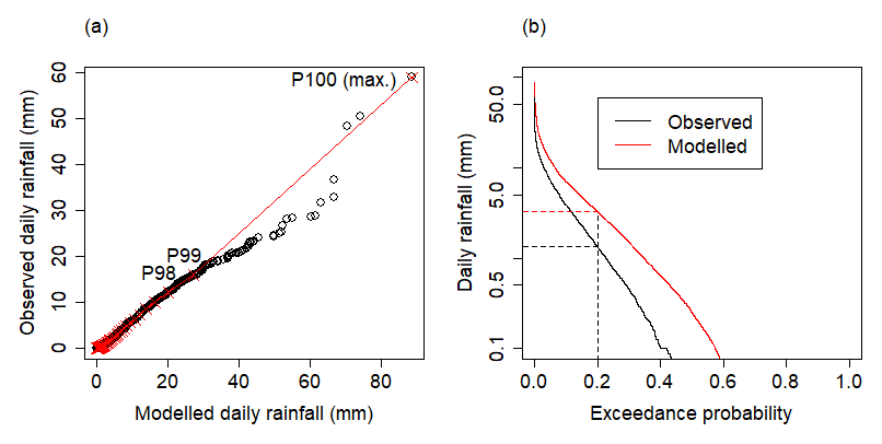
Figure 1Schematic of QQM bias correction. (a) Empirical cumulative density functions for both observed and modelled rainfall in a given grid cell. Percentiles are estimated from both distributions, which are equated in bias correction to generate a mapping function (b). Values lying between percentiles or outside the modelled maximum value are interpolated or extrapolated linearly.

Download

2.4 Defining transition probabilities

Whereas QQM bias correction can correct the daily distribution exactly, daily bias correction is not set up to correct sequences and accumulations (Addor and Seibert, 2014). To this end, we consider not only how bias correction affects daily metrics of rainfall but also the sequencing of wet days that produce runoff. One way of measuring this is through transition probabilities of wet and dry sequences. To this end, we consider a simple two-state Markov chain rainfall occurrence model. Here, the probability of a wet or dry day depends on whether the previous day was wet or dry. A “dry” day can be defined as either zero rainfall or rainfall below a given threshold (such as 1 mm). Define the wet-to-wet transition probability (i.e. the probability of a wet day following a wet day) as $w=\mathrm{Pr}\left(W_n\mathrm{|}{W}_{n-\mathrm{1}}\right)$ and the corresponding dry-to-dry transition probability as $d=\mathrm{Pr}\left(D_n\mathrm{|}{D}_{n-\mathrm{1}}\right)$. These determine the Markov chain since $\mathrm{Pr}\left(D_n\mathrm{|}{W}_{n-\mathrm{1}}\right)=\mathrm{1}-w$ and $\mathrm{Pr}\left(W_n\mathrm{|}{D}_{n-\mathrm{1}}\right)=\mathrm{1}-d$. Further, the probability of the occurrence of a dry day, p, is fully determined by the w and d parameters, as given by Cox and Miller (1965):

Equivalently,

This relationship can be plotted for a range of probabilities p (dotted lines in Fig. 10). Note that, if a series of occurrences of dry and wet days has zero autocorrelation (i.e. the state probability is independent of the rainfall state in the previous day), then it follows that $\mathrm{Pr}\left(D_n\mathrm{|}{D}_{n-\mathrm{1}}\right)=\mathrm{Pr}\left(D_n\mathrm{|}{W}_{n-\mathrm{1}}\right)=\mathrm{Pr}\left(D_n\right)=p$. As such, the diagonal line where p=d (dashed line in Fig. 10) corresponds to an independent (i.e. zero autocorrelation) series of occurrences. The area above and to the right of the dashed line corresponds to a series of occurrences with positive autocorrelation (i.e. $\mathrm{Pr}\left(D_n\mathrm{|}{D}_{n-\mathrm{1}}\right)>p$, so that dry sequences are more likely to persist), whereas the area below and to the left of the dashed line corresponds to series with negative autocorrelation. The framework developed above is used in Sect. 3.3 as a novel way to represent the relationships between state transition probabilities and rainfall quantiles to investigate the effect of bias correction on transition probabilities.

3.1 Assessment of regional performance of modelled rainfall

Modelled rainfall is compared to observed (AWAP) rainfall in Fig. 2. ECHAM5-R1 was chosen as a representative GCM–RCM ensemble member here as it had the median historical regional rainfall across Victoria from the NARCliM model ensemble. The spatial rainfall fields downscaled from both the reanalysis and GCM both show reasonable agreement with the spatial pattern of the observed mean annual rainfall, with relatively larger rainfall across the mountain ranges to the east of the state and across the southern coast, and less rainfall to the more arid north-west region. However, both rainfall fields are evidently positively biased with around 100–200 mm of excess rainfall consistently across most of the state (Fig. 2f, g), and relatively more for the far eastern part of Victoria for the reanalysis data and across the mountain ranges for the GCM data, interspersed with small patches of negative bias (observations larger than downscaled data). Averaged across Victoria, the mean absolute bias is approximately 26 % for the downscaled reanalysis and 43 % for the downscaled GCM data. In comparison, the absolute change signal averages 3 %, rising to around 10 % in the eastern part of Victoria (Fig. 2h).

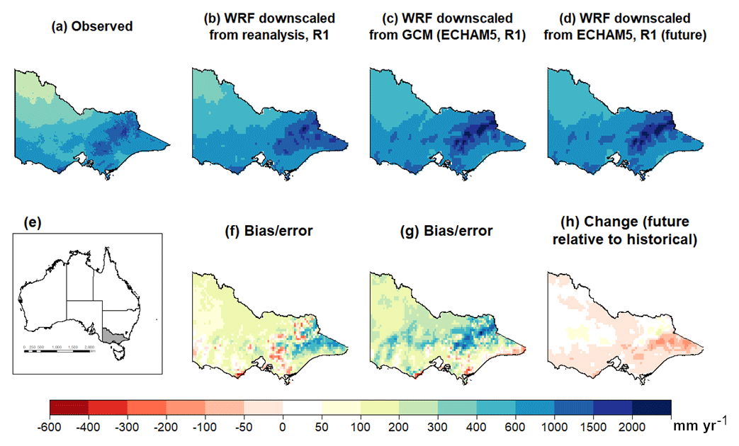
Figure 2Regional mean annual rainfall (mm yr⁻¹). Inset map (e) shows the location of the state of Victoria in Australia. Other panels show (a) observed (AWAP) rainfall, (b) rainfall downscaled from reanalysis (NCEP/NCAR), (c) historical rainfall downscaled from median GCM (ECHAM5-R1), (d) future rainfall downscaled from GCM, (f) bias in reanalysis downscaling (compared to observed), (g) bias in GCM downscaling and (h) change factor of GCM downscaled rainfall.

3.2 Bias correction of NARCliM

Consistent with Fig. 2, the raw NARCliM rainfall is mostly wetter (positive bias) across Victoria (Fig. 3a), except for a tendency towards underprediction in the south-east coast for some models. The quantile–quantile bias-correction method is formulated to correct historical quantiles of rainfall exactly (when applied to the same time period used for calibration) so that bias-corrected mean annual rainfall, as well as any quantiles, is approximately equal (Fig. 3b). However, the method used here does not correct high rainfall quantiles (e.g. P99 and above) exactly, due to the interpolation between quantiles as described in Sect. 2.3 (Fig. 4b). This residual bias appears to be randomly distributed spatially and results in bias-corrected mean annual rainfall not being exactly corrected. However, this effect is generally less than 5 % of the mean annual rainfall. This effect can be removed entirely by using empirical density functions rather than interpolated values, but with the effect of increasing prediction uncertainty.

Figure 3Percentage bias in WRF-downscaled mean annual rainfall from the GCM/RCMs indicated (a) raw data and (b) residual bias (after bias correction).

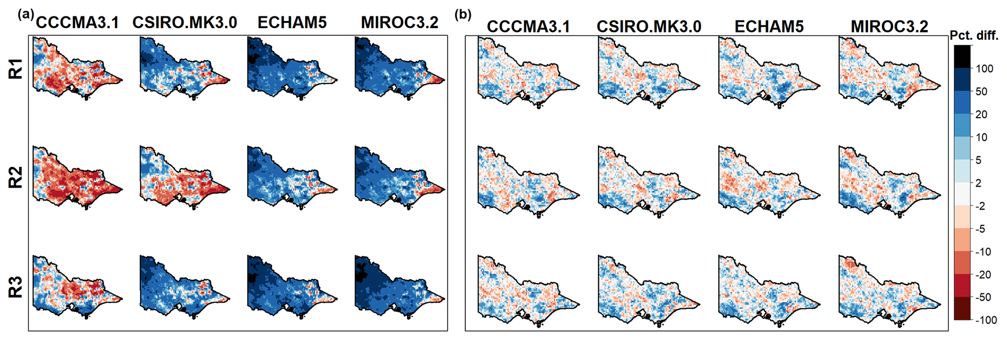
Figure 4Percentage bias in WRF-downscaled 99th percentile of rainfall (P99) from the GCM/RCMs indicated (a) raw data and (b) residual bias (after bias correction).

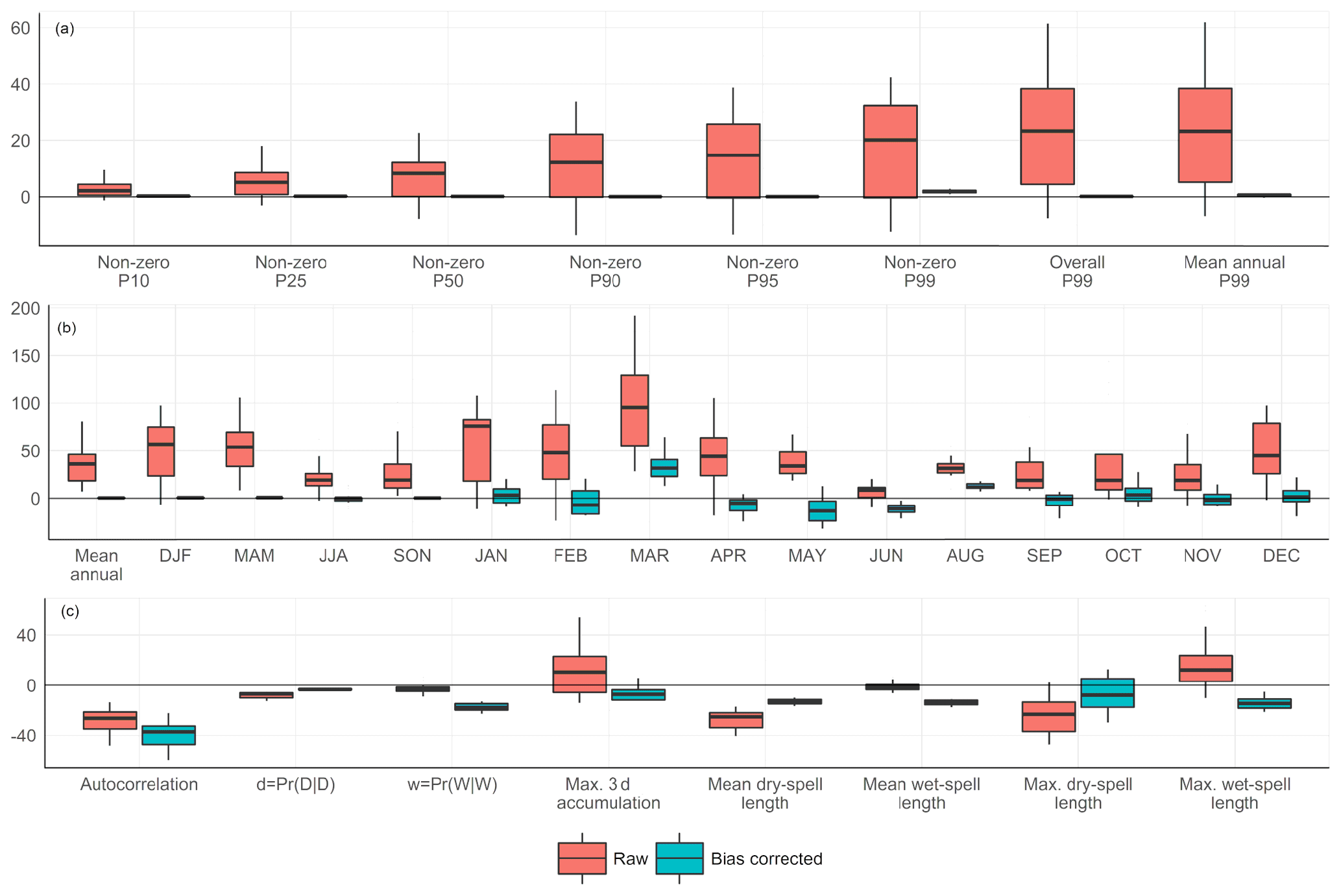
Figure 5Relative bias (modelled compared to AWAP, as percentages) of (a) rainfall percentiles; (b) mean annual, seasonal and monthly rainfall; and (c) rainfall-sequencing metrics both before and after bias correction. The range of results represents the spread of downscaled GCM hindcast spatial averages over Victoria from the NARCliM 12-model ensemble.

Download

Figure 5 shows the distribution of bias for different rainfall metrics before bias correction and the residual bias after QQM bias correction. The bias in raw NARCliM ranges from 5 to 50 % for all percentiles (Fig. 5a), increasing as the percentile increases (i.e. more relative bias for higher rainfall amounts). As with Fig. 3, bias at all percentiles is effectively reduced to zero after bias correction, although the residual bias is relatively larger at larger percentiles (higher rainfall), similarly to Fig. 4b. NARCliM rainfall is overestimated at all seasons and months before bias correction (Fig. 5b), although winter rainfall is relatively less biased than summer rainfall. Bias correction reduces bias to zero annually and seasonally, since QQM is applied to each season separately. Since the intra-seasonal relative monthly rainfall amounts are not exactly equal to the observed amounts, seasonal bias correction occasionally overcorrects bias, particularly in February, April, May and June, with the bias-corrected rainfall in these months being less than observed whereas they were overpredicted before bias correction; this could be reduced to zero using monthly correction factors, although at the potential cost of overfitting. Overall though, the absolute relative bias is reduced and closer to zero in all months compared to the raw RCM monthly amounts.

Figure 6Biases in spatial average 3 d rainfall accumulation percentiles. Here a 3 d moving-average filter was applied to each hindcast time series and equivalent quantiles taken at increasing probability values (x axis).

Download

Figure 5c shows relative bias in rainfall-sequencing-related metrics. Autocorrelation of rainfall amounts is underpredicted before bias correction, and the magnitude of this bias actually increases after bias correction. Whereas QQM reduces bias in dry–dry transition probabilities (i.e. the probability of dry sequences persisting), bias in wet–wet transition probabilities increases after bias correction so that, similarly to autocorrelation, the probability of wet spells persisting is considerably underpredicted after bias correction. We examine this in more detail in Sect. 3.3 using the transition probability framework developed in Sect. 2.4. Since dry spells are directly related to dry–dry transition probabilities, the bias in mean and maximum dry spells is well corrected, whereas maximum 3 d rainfall accumulation and wet-spell occurrences all have negative bias after QQM bias correction. Different percentiles of 3 d rainfall accumulation (calculated as percentiles of a 3 d moving sum of rainfall time series) have different residual bias (Fig. 6). Three-day accumulation percentiles below the 80th are all slightly overestimated after bias correction, but above the 80th percentile a large residual underestimation is present. This underestimation reduces at around the 99th percentile but is moderated somewhat for the 3 d maximum (i.e. 100th percentile). As noted in Sect. 2.1, WRF models were selected according to their skill in reproducing selected 2-week periods of heavy rainfall. This provides a potential explanation for the smaller bias in 3 d maxima relative to 3 d 99 % rainfall.

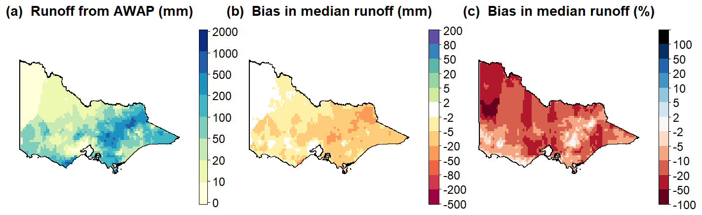
Figure 7Ensemble (downscaled GCM hindcasts from the NARCliM 12-model ensemble) median modelled runoff over Victoria: (a) from AWAP historical observations, (b) absolute bias (mm) and (c) percentage bias (%).

It is likely that underpredicting wet-spell occurrences and persistence (Figs. 5c and 6) will result in runoff from the bias-corrected rainfall being underpredicted too. To explore this, runoff was modelled from bias-corrected rainfall and observed potential evapotranspiration data using GR4J (see Charles et al., 2020, for more details). Figure 7 plots the percentage difference in bias-corrected ensemble-median mean annual runoff for each $\mathrm{0.1}{}^{\circ }\times \mathrm{0.1}{}^{\circ }$ cell compared to mean annual runoff modelled using AWAP-observed rainfall. The ensemble median of runoff across Victoria is underpredicted by 10–20 % across almost all of Victoria, which suggests that the residual bias in wet-spell occurrences and persistence is problematic for runoff modelling. Whereas the smallest percentage biases appear to be over the high-runoff-producing region (Fig. 7c), this region has the highest absolute biases with bias in runoff of more than −20 mm (Fig. 7b). Characteristics and biases of runoff from bias-corrected NARCliM rainfall is explored in more detail by Charles et al. (2020).

3.3 Residual bias in rainfall state transition probabilities

The results in this study demonstrate that dry–dry transition probabilities for NARCliM have low residual bias (possibly due to the emphasis in QQM on preserving zero-rain occurrences) but that wet–wet transition probabilities have more bias (i.e. they are closer to zero; see Fig. 5c) after QQM bias correction. These residual biases in wet–wet transitions result in the persistence of wet spells being underestimated even though the volumetric amount of rainfall is, by design of QQM bias correction, equal to observed rainfall at any grid point.

Figure 8Dry–dry transition probabilities (1 mm threshold).

After bias correction, dry–dry transition probabilities for a 1 mm threshold are reduced but still have a small negative bias (Fig. 5c). Both the bias-corrected WRF-downscaled reanalysis and bias-corrected WRF-downscaled GCM results (Fig. 8) show a spatial pattern very similar to observations with higher dry–dry transition probabilities to the north-west of the state and at similar places along the southern coastline. However, the reanalysis and more so the GCM result have a lower dry–dry transition probability across almost all of the region (Fig. 8). As such, dry spells from the bias-corrected model output are likely to be shorter in duration and less common than those from the observed rainfall (although bias correction does reduce the bias in dry spells somewhat compared to the bias in the raw data as seen in Fig. 5c).

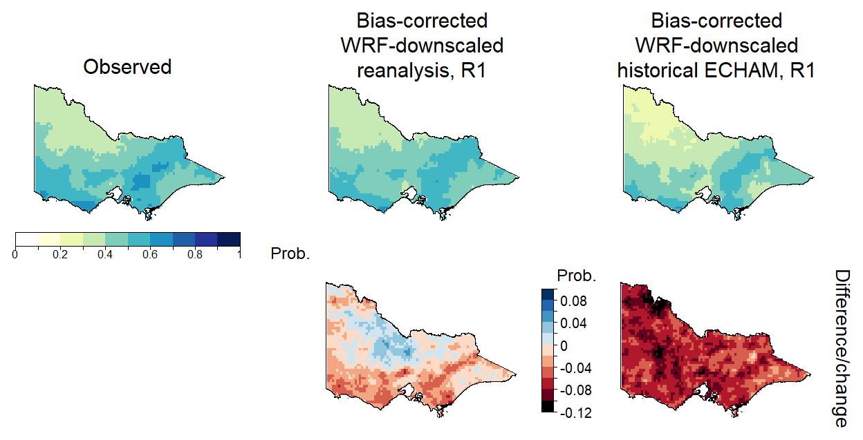
Figure 9Wet–wet transition probabilities (1 mm threshold).

Whereas the dry–dry transition probabilities were largest in the north-west, drier, part of Victoria, the wet–wet transition probabilities are largest over the high-runoff-producing region (Fig. 9), which corresponds to the high-relief, high-altitude part of the state. As with the dry–dry transition probabilities, both bias-corrected downscaled reanalysis and bias-corrected downscaled GCMs reproduce the spatial pattern of wet–wet transition probabilities, but there is considerable residual bias in these probabilities across the entire region. The residual bias in WRF-downscaled GCM transition probabilities is over 10 % over most of Victoria. This residual bias results in underestimation of wet-spell occurrences and durations and multi-day accumulations of rainfall (Fig. 5c). The bias in wet–wet transition probabilities is more problematic for modelling runoff than the bias in dry–dry transition probabilities, not only because it is of larger magnitude but also because runoff is sensitive to multi-day wet spells, and the larger wet–wet probabilities occur in high-runoff-producing areas, which we would like to model correctly for regional water availability projections.

Figure 10 shows rainfall percentiles for a sample grid cell overlaid on the transition-probability space developed in Sect. 2.4. Other grid cells and GCMs show very similar responses (as can be seen in the low spread of results for d and w in Fig. 5c). Quantile–quantile mapping bias correction equates the quantiles for each rainfall amount such that equal rainfall amounts for observations and bias-corrected rainfall occur on the same probability contours (dotted lines in Fig. 10), with raw values translated along the rainfall amount curve. That is, values on the blue line in Fig. 10 map to corresponding values on the red line; the slight variation between the lines is due to different bias corrections in each season. As such, wet–wet and dry–dry transition probabilities for a given rainfall threshold (e.g. 1 mm) for bias-corrected rainfall are equal to the transition probabilities for the corresponding amount in the raw data. For example, in Fig. 10, the exceedance probability for 1 mm in the observed data (green line) is 0.774. The corresponding quantile in the raw data (blue line) is 2.675 mm. This amount is mapped to 1 mm in the bias-corrected data (red line), and the corresponding wet–wet and dry–dry transition probabilities for 2.675 mm are identical to the transition probabilities for 1 mm in the bias-corrected data. Recall that points above and to the right in Fig. 10 correspond to more (positive) serial correlation, which means that the observed rainfall time series contains more correlation structure in the sequence of wet- and dry-spell occurrences than the modelled rainfall sequence, and that QQM bias correction cannot rectify this since daily QQM retains the autocorrelation structure of the raw time series since daily amounts are simply rescaled. We surmise that, as bias correction is ultimately intended to produce physically plausible rainfall, bias-correction methods that adjust occurrences are needed to properly correct biases for hydrological modelling.

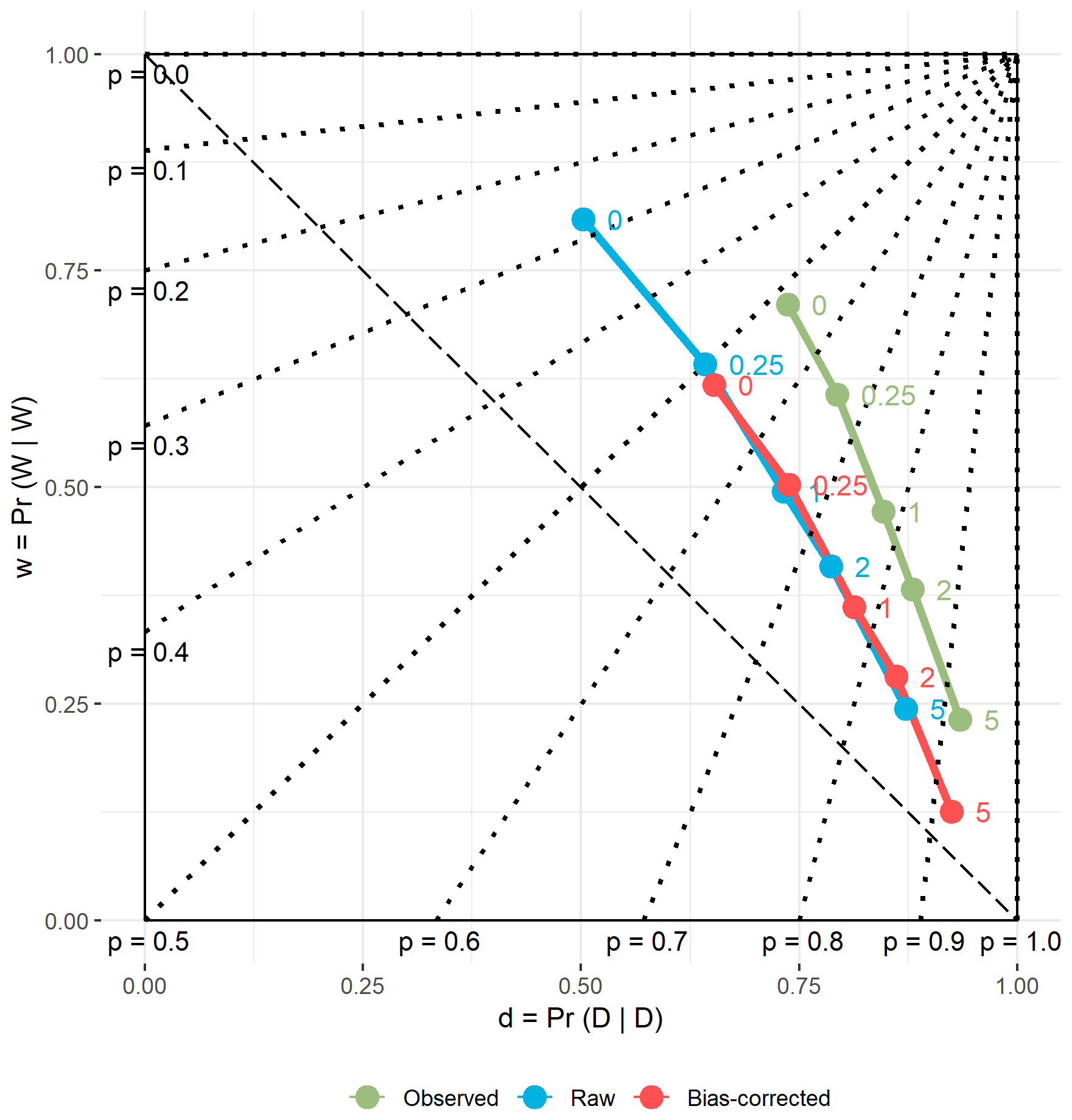
Figure 10An alternative perspective on quantile–quantile mapping: daily rainfall amounts and associated probabilities plotted in d–w space. Quantile–quantile mapping bias correction (red) maps daily rainfall amounts from the raw data (blue) to the probability contours (dotted lines) corresponding to the appropriate observed daily amount (green). The dashed diagonal line represents p=d and hence an independent series of events (see Sect. 2.4). Points lying above or to the right represent quantiles with greater (more persistent) autocorrelation.

Download

3.4 Change signals

Here we examine change signals in rainfall metrics (i.e. percentage difference in RCM future relative to RCM historical averages), specifically looking at whether bias correction alters the change signals. Figure 11a shows the change signals in different rainfall percentiles. For the raw data, there is a small decrease in low to moderate rainfall amounts less than the non-zero 40th percentile and a future increase in non-zero percentiles above 50 %. The nature of QQM bias correction means that raw and bias-corrected equal percentiles cannot be meaningfully compared. Nevertheless, a similar pattern is found with the bias-corrected data, namely that larger rainfall amounts have larger relative changes than smaller rainfall amounts.

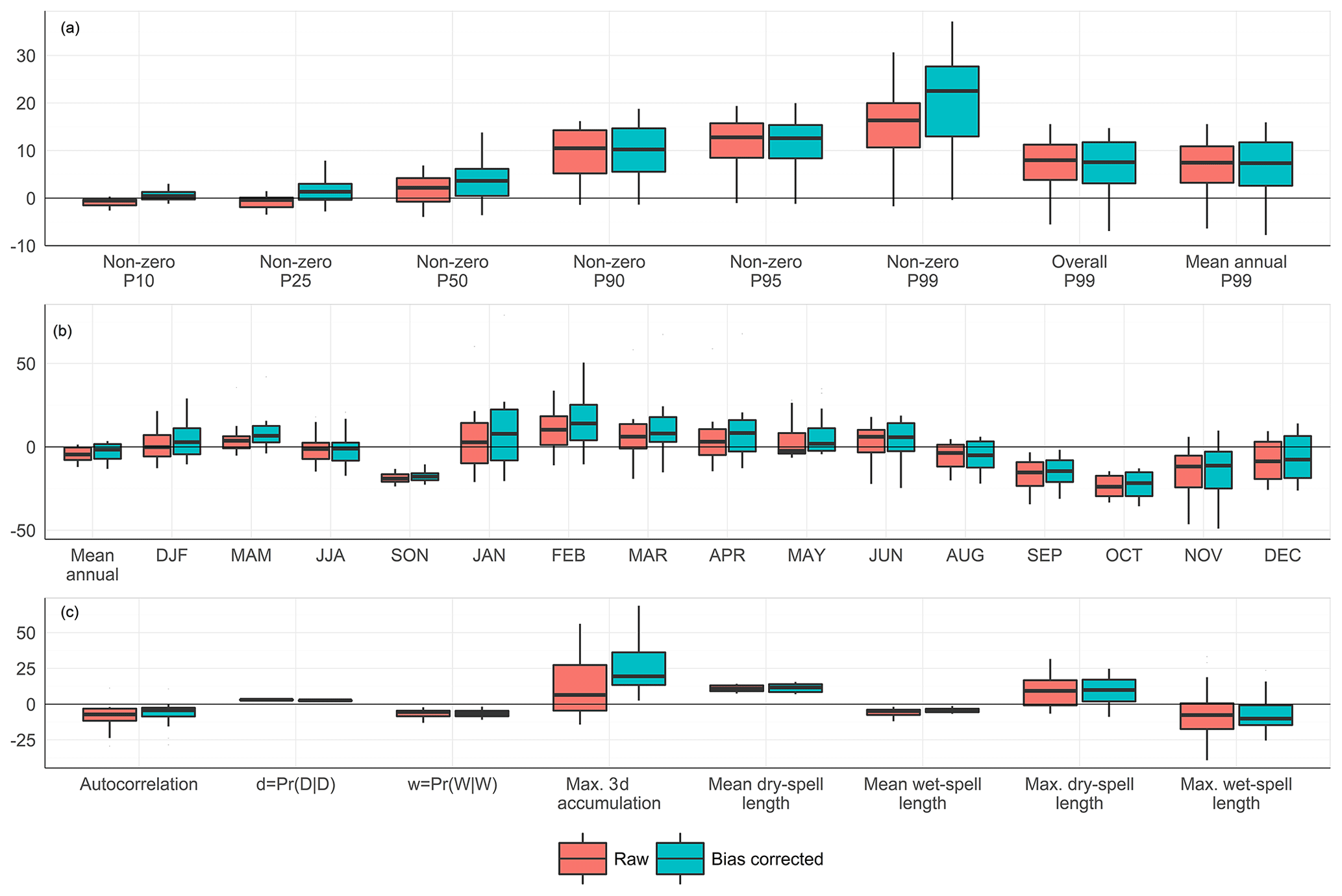
Figure 11Change signal (percentage difference of RCM future relative to RCM historical) in (a) rainfall percentiles; (b) mean annual, seasonal and monthly rainfall; and (c) rainfall-sequencing metrics both before and after bias correction.

Download

Figure 11b shows change signals in mean annual, seasonal and monthly average rainfall. The magnitude of the median change signal in mean annual rainfall is around −5 %, and seasonal changes are comparable to the annual change except for SON rain. Rain in SON has a decrease projected by the NARCliM ensemble of around 20 % (found to be statistically significant by Olson et al., 2016). Compared to the raw bias in mean and seasonal rainfall (Fig. 5b) of 25–50 %, these change signals are between 1∕2 and 1∕10 of the bias. After bias correction, there is little difference in the magnitude and direction of change in seasonal and monthly averages. However, the mean annual rainfall change is moderated somewhat, and this is problematic since mean annual changes are most often considered in regional projection applications (a discussion on bias-correction effects on change signals is considered in the next section, and Charles et al. (2020) discuss this in the context of the present study in more detail).

Although the residual bias in rainfall sequencing metrics is not eliminated, and in some cases (e.g. wet–wet transition probabilities) is actually increased, after bias correction (Fig. 5c), Fig. 11c shows that the change signals in rainfall sequencing metrics is largely unaffected by bias correction. With the exception of the maximum accumulation of rainfall over 3 d rainfall accumulation, the distributions of sequencing change signals are largely identical before and after bias correction. The difference in change signal for maximum 3 d rainfall accumulation is presumably related to the relatively larger increase in large rainfall events (e.g. P99 in Fig. 11a).