the Creative Commons Attribution 4.0 License.
the Creative Commons Attribution 4.0 License.
 | 08 Jun 2020
Impact of downscaled rainfall biases on projected runoff changes
Stephen P. Charles
Francis H. S. Chiew
Nicholas J. Potter
Hongxing Zheng
Guobin Fu
Lu Zhang
Realistic projections of changes to daily rainfall frequency and magnitude, at catchment scales, are required to assess the potential impacts of climate change on regional water supply. We show that quantile–quantile mapping (QQM) bias-corrected daily rainfall from dynamically downscaled WRF simulations of current climate produce biased hydrological simulations, in a case study for the state of Victoria, Australia (237 629 km2). While the QQM bias correction can remove bias in daily rainfall distributions at each 10 km × 10 km grid point across Victoria, the GR4J rainfall–runoff model underestimates runoff when driven with QQM bias-corrected daily rainfall. We compare simulated runoff differences using bias-corrected and empirically scaled rainfall for several key water supply catchments across Victoria and discuss the implications for confidence in the magnitude of projected changes for mid-century. Our results highlight the imperative for methods that can correct for temporal and spatial biases in dynamically downscaled daily rainfall if they are to be suitable for hydrological projection.
- Article
(1040 KB) - Companion paper
-
Supplement
(149 KB) - BibTeX
- EndNote


Modelled hydrological response to climate change, conditioned on regional climate projections, can inform water supply planning for resilience on multi-decadal and longer timescales. Global climate models (GCMs) provide broadscale projections (length scales of 100+ km) that are too coarse for direct use in hydrological modelling; hence GCMs are often dynamically downscaled using regional climate models (RCMs) to provide regional (∼10 km length scale) projections. RCMs can better capture the spatial variability in rainfall change at the scale of catchment response, particularly where there is high spatial variability in rainfall due to orography (Ekström et al., 2015; Grose et al., 2015; Casanueva et al., 2016; Di Luca et al., 2016; Rummukainen, 2016). However, RCM rainfall characteristics such as daily distributions and sequencing often do not match observations sufficiently well for them to be used directly as input to hydrological models (Maraun et al., 2010; Ehret et al., 2012; Rasmussen et al., 2012; Muerth et al., 2013; Räty et al., 2014). Thus, “bias-correction” (BC) methods are commonly applied to adjust RCM rainfall output to match certain characteristics of the observed rainfall (Teutschbein and Seibert, 2012). There is no “perfect” bias-correction approach; thus subjective decisions on their application together with methodological limitations are a source of uncertainty in bias-corrected RCM rainfall and the resulting hydrological changes simulated using them (Lafon et al., 2013; Teutschbein and Seibert, 2013; Teng et al., 2015; Ivanov and Kotlarski, 2017; Maraun and Widmann, 2018; Potter et al., 2018). Reported limitations of many daily rainfall bias-correction methods include the inability to correct for biases in multi-day rainfall totals, or the daily sequencing of wet and dry days (Chen et al., 2013; Addor and Seibert, 2014; Evans et al., 2017). More generally, bias correction cannot correct for RCM errors inherited from GCM errors in seasonality, temporal sequencing or large-scale circulation biases that could result in unphysical climate projections (IPCC, 2015). Bias correction also assumes stationarity in the quantile–quantile mapping (QQM) relationship, assuming that the mapping derived for the historical period applies under future climate conditions (Teutschbein and Seibert, 2013).
There is also debate and uncertainty due to the modifications in the climate change signal (CCS) caused by the bias correction (Ivanov and Kotlarski, 2017; Hagemann et al., 2011; Dosio et al., 2012; Themeßl et al., 2012; Velázquez et al., 2015; Mbaye et al., 2016; Switanek et al., 2017; Ivanov et al., 2018; Sangelantoni et al., 2018). Teng et al. (2015) determined that bias correction altered the change signal for many characteristics, including high rainfall amounts, which had a significant impact on simulated runoff and particularly high flows. Ivanov et al. (2018) examined this issue and concluded that the bias-corrected CCS resulting from correcting RCM intensity distribution bias is defensible.
Here we report on the impact that bias-correcting daily rainfall from WRF (Weather Research and Forecasting regional climate model) has on the characteristics of projected future runoff (i) across the state of Victoria in south-east Australia and (ii) in more detail for 10 catchments within Victoria. Potter et al. (2020) found that the QQM bias-correction approach used to correct WRF-raw daily rainfall, applied on a cell-by-cell seasonal basis, does not correct for underestimation biases in wet–wet transition probabilities. Hence, as we show, WRF-BC rainfall will tend to underestimate runoff compared to runoff simulated using observed rainfall. At the catchment scale both raw and WRF-BC rainfall underestimate spatial correlation between cells within a catchment, which is an additional source of runoff uncertainty. Similar results and limitations have been observed for various BC methods in the literature (Lafon et al., 2013; Teng et al., 2015; Maraun, 2016; Rajczak et al., 2016; Maraun et al., 2017).
The state of Victoria in south-eastern Australia (Fig. 1) experiences mild wet winters and hot dry summers, with large interannual-to-decadal climate variability producing a significant impact on water availability for agriculture and water supply for towns and cities (Kiem and Verdon-Kidd, 2010; Chiew et al., 2014, 2018). Higher runoff is produced in highland (Victorian Alps) and coastal catchments along southern and eastern coastlines. Low-runoff catchments are in the inner western regions and western slopes of the Great Dividing Range (Hope et al., 2017). Rainfall is projected to decline across the state, together with increased intensity of extreme rainfall events (DELWP, 2019).

Figure 1State of Victoria, Australia, mean annual rainfall for AWAP for 1990–2009 and location of study catchments used for rainfall–runoff modelling.
Given these sensitivities to climate variability and change, a research partnership (Victorian Climate Initiative, VicCI) between Victoria's state government (Department of Environment, Land, Water and Planning: DELWP) and Australian research organisations (Bureau of Meteorology and CSIRO) was initiated to ensure that water policies and management decisions were informed by the most up-to-date earth systems and climate change science (Hope et al., 2017). VicCI produced projections using daily empirical scaling (Potter et al., 2016). In this study we investigate QQM-BC dynamically downscaled WRF rainfall simulations for their ability to reproduce simulated runoff for observed conditions across the whole state of Victoria and also, in more detail, for 10 water supply catchments selected on the basis of their hydrological model performance in reproducing reference runoff (study area and catchments shown in Fig. 1). The QQM-BC approach, using the R package “qmap” using the methodologies developed by Gudmundsson et al. (2012), is applied for each 3-month season (i.e. DJF, MAM, JJA and SON) to each grid cell independently, mapping the simulated (WRF) to the observed (AWAP) daily rainfall cumulative density function quantiles such that a WRF-simulated amount is replaced with the observed rainfall amount for the corresponding percentile, with linear interpolation between percentiles and for upper-tail simulated amounts greater than observed.
Thus, we investigate the historical performance and CCS of runoff simulated from
- a.
WRF-raw rainfall.
- b.
WRF-BC rainfall (BC, by season, using QQM).
- c.
Observed rainfall that was empirically scaled according to annual WRF-raw rainfall changes. For observed rainfall we use AWAP (Australian Water Availability Project) 5 km × 5 km gridded daily climate data, available Australia wide, interpolated from station data (Jones et al., 2009). The 5 km × 5 km AWAP daily rainfall was resampled to the 10 km × 10 km WRF grid and then empirically scaled by the WRF change annual factor, to give future rainfall. This empirical scaling method (Chiew et al., 2009) rescales the historical grid-cell time series by multiplicatively applying the changes between historical and future period climate model projections. This can be applied on an annual basis, on a seasonal basis, or in a two-step process first on a seasonal and then on an annual to maintain the overall annual change as projected by the climate model.
- d.
Observed (AWAP) rainfall that was empirically scaled according to seasonal WRF-raw rainfall changes and then rescaled to match annual WRF-raw rainfall changes.
- e.
The seasonal WRF-BC rainfall from (b) twice rescaled to firstly match WRF-raw seasonal rainfall changes and then additionally rescaled to match WRF-raw annual rainfall changes.
As (a), (c), (d) and (e) have the same annual rainfall changes, this allows us to assess the impact on runoff projections of the choices of using BC versus empirical scaling. We show how the mean, high- and low-flow change characteristics are influenced by these choices.
2.1 Downscaled inputs to hydrological modelling
As a pragmatic choice due to their ready availability, we use downscaled simulations from the NARCliM (NSW and ACT Regional Climate Modelling) project (http://www.ccrc.unsw.edu.au/sites/default/files/NARCliM/index.html, last access: 2 June 2020). Evans et al. (2014) described the experimental design for these WRF-downscaled simulations, outlining the selection of four Coupled Model Intercomparison Project Phase 3 (CMIP3) GCMs (CCCM3.1, CSIRO-Mk3.0, ECHAM5 and MIROC3.2 (medres)) based on a three-stage process: (1) the performance of a total of 23 CMIP3 GCMs was evaluated, and models that did not adequately simulate the historical climate of south-eastern Australia were rejected; (2) the set of GCMs that performed well was then ranked on the basis of a measure of their independence; and (3) the GCMs were then evaluated on the basis of their projections of future climate change. The four most independent models that spanned the largest range of plausible future climates were chosen. These GCMs were used for the boundary conditions for producing future projections and three WRF configurations (R1, R2 and R3) that vary the combinations of planetary boundary layer, surface layer, cumulus and short-wave/long-wave radiation physics used. Note that ongoing WRF research is using CMIP5 GCMs, but these results were not available to us within the time frame of the current project. Also, other RCMs could produce different results when forced by the same GCMs.
Ji et al. (2016) assessed the three WRF configurations, driven by NCEP/NCAR Reanalysis boundary conditions, against AWAP (Jones et al., 2009) observations. They concluded that the R2 simulations performed best in terms of reproducing rainfall seasonal cycles, interannual and decadal variability and spatial patterns over southeast Australia, while noting biases in rainfall amounts can be substantial in some seasons and regions. Olson et al. (2016) also referred to significant WRF biases in rainfall climatology, noting that this was not surprising given WRF configuration selection was on the basis of skill for selected storm events of 2-week periods, rather than performance at the climatological scale.
Given these findings, we have used WRF-BC R2 simulations over Victoria for reanalysis (NCEP/NCAR and ERA-Interim for 1990–2009) and GCM historical (for 1990–2009) and future Special Report on Emissions Scenarios (SRES) A2 (for 2060–2079) forced simulations. The SRES A2 scenario describes a very heterogeneous world with high population growth and technological change that is fragmented and slow (Nakicenovic et al., 2000). The SRES A2 emission scenario was selected for the NARCliM climate projections because the global emissions trajectory suggested that it was the most likely scenario. Recent publications have confirmed that we are tracking at the higher end of the A2 scenario (Peters et al., 2013). Whilst the SRES A2 is from the previous generation of CMIP3 scenarios (Nakicenovic et al., 2000), it is relevant to assessing plausible climate change impacts as Woldemeskel et al. (2016) have shown that CMIP3- and CMIP5-projected precipitation changes are similar for southern Australia.
Note we have only assessed the impact of WRF rainfall bias correction and changes, using AWAP-derived mean-monthly daily potential evapotranspiration (PET) in all cases, to allow us to examine the impact of rainfall properties and changes in isolation from other confounding factors such as temperature and PET change. Changes to PET would cause an additional reduction in runoff under a warming climate but would not change the relative results, as presented, in any considerable manner because the range of change is dominated by the large range in rainfall projections; i.e. PET is a second-order effect. For example, for a similar region Potter and Chiew (2011) found increased PET only explained 5 % of runoff reduction in a prolonged drought. We have designated the rainfall simulated by WRF model as “raw” rainfall, to differentiate from the bias-corrected rainfall (henceforth designated “BC rainfall”). The resulting runoff, simulated using the raw or BC rainfall inputs, is thus designated “raw runoff” or “BC runoff”; note that “BC” refers to the use of bias-corrected rainfall inputs to rainfall–runoff modelling.
2.2 Hydrological model
We undertook the hydrological modelling experiments using the GR4J rainfall–runoff model (Perrin et al., 2003). The GR4J model is based on the unit hydrograph principle and has been found to be competent in hydrological simulation for a large number of catchments globally. It has four parameters representing maximum capacity of the soil moisture storage (x1), interbasin water exchange rate (x2), maximum routing storage (x3) and time base of unit hydrographs (x4).
In this study, for rainfall–runoff simulation at each grid cell, the GR4J model was first calibrated against observed daily streamflow at 137 unimpaired catchments in the region for the period 1981–2010 (for calibration details see Figs. S1 and S2 in the Supplement). The calibrated parameters are then applied for each grid cell in Victoria using the nearest-neighbour parameter sets (Chiew et al., 2017, 2018). Since each grid cell is considered as an independent catchment for the investigation, channel routing describing the connection between the grid cells is not applied in this case. The objective function of model calibration is defined as
where
where NSE is the Nash–Sutcliffe efficiency, Qmod is modelled daily streamflow, Qobs is observed daily streamflow, is mean modelled streamflow, is mean observed streamflow and n is total number of days in the modelling period. This objective function, from Viney et al. (2009), combines the commonly used NSE and the bias to constrain total model bias in runoff simulation.
Additionally, for a catchment-scale investigation regarding spatial correlation of rainfall within the catchment, two methods for rainfall–runoff model calibration are compared, a “distributed” method and a “lumped” method. For the distributed method, simulations are run for each 10 km × 10 km grid cell within each catchment using BC rainfall as input, and the runoff simulated for the cells is averaged (with proportional weighting for cells partially within the catchment) to produce catchment-mean runoff, which is then assessed against the AWAP-simulated daily streamflow (millimetres per day) at the outlet gauge of the catchment. For the lumped method, GR4J is calibrated using a single areal mean daily rainfall time series obtained by averaging AWAP rainfall for the grid cells within the catchment (with proportional weighting for cells partially within the catchment). Corresponding BC lumped rainfall from WRF is used as the input to GR4J to simulate runoff for each catchment.
3.1 Historical simulations
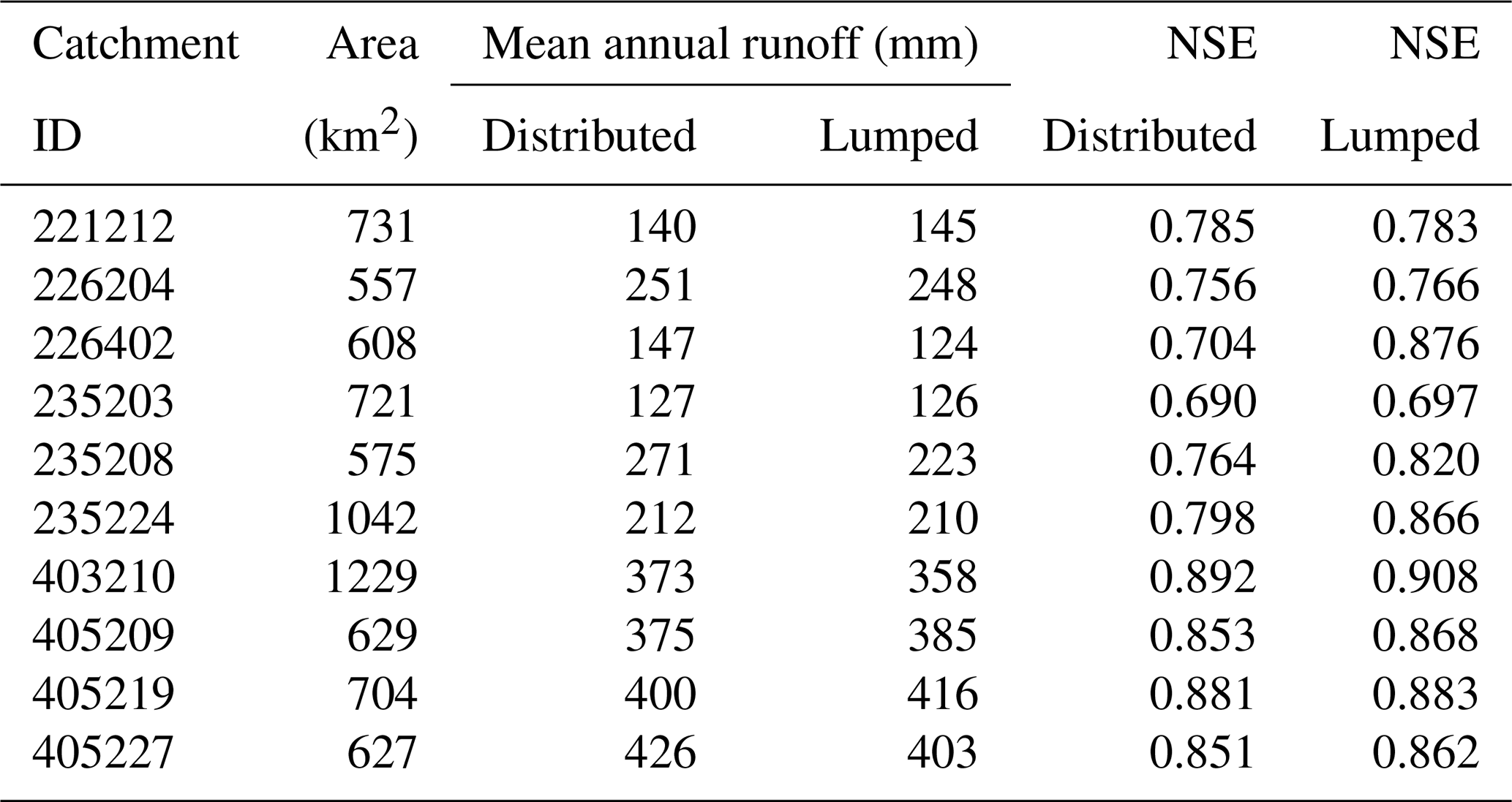
Table 1 shows that calibration results of the two methods are comparable at most of the 10 catchments. It is interesting to note that the mean annual runoff from the distributed modelling is generally slightly greater than the runoff from the lumped modelling and that the lumped modelling generally produced a slightly better calibration than the distributed modelling. Such results are consistent with the findings of Andréassian et al. (2004). The reason the distributed modelling produces slightly higher runoff is it overweights the runoff contribution from the grids with higher precipitation. In the lumped modelling, the catchment-mean precipitation filters out rainfall intensity in some grids; hence the intensity signal is attenuated and produces less runoff.
Table 1Catchment attributes and distributed and lumped calibration (1990–2009 period) runoff and NSE metrics.
Hereafter, we use the term “reference” runoff simulations where AWAP rainfall and PET for the 1990–2009 period were inputs to the GR4J model. The reference runoff simulations were considered the benchmark to assess the simulated runoff using dynamically downscaled WRF-BC rainfall for reanalysis-forced and GCM-forced historical runs for the 1990–2009 period. WRF-BC rainfall for GCM-forced 2060–2079 runs were used to produce simulated projections of future runoff.
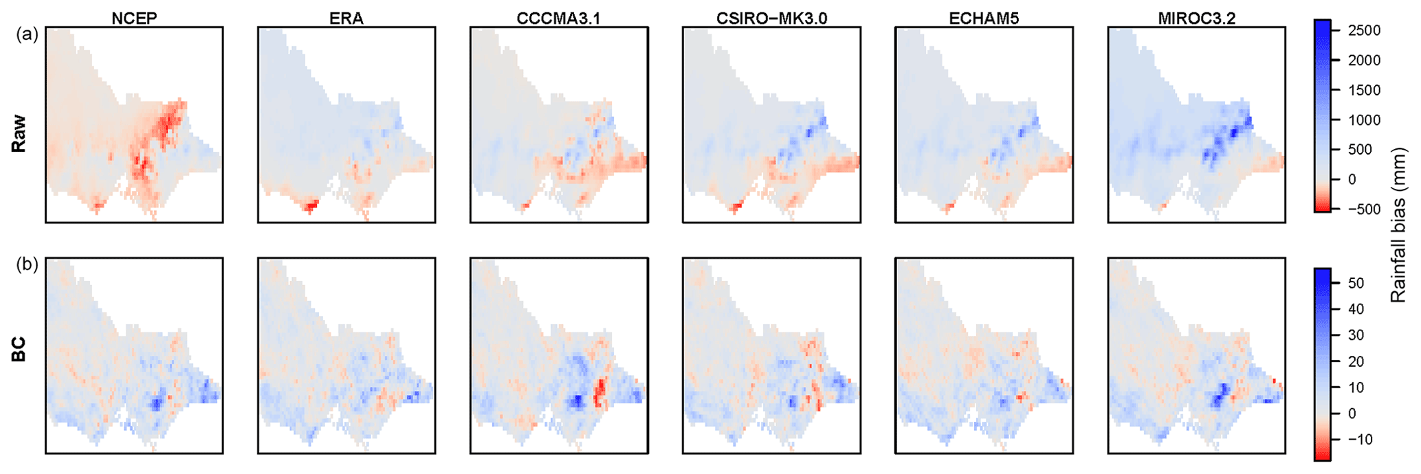
Figure 2Historical (1990–2009) mean annual rainfall bias (WRF minus AWAP, mm) for (a) WRF-raw and (b) WRF-BC. Columns (left to right) are WRF runs forced by two reanalyses (NNR and ERAI) and then four GCMs (CCCMA3.1, CSIRO-MK3.0, ECHAM5 and MIROC3.2).
The WRF-raw rainfall was found to have large absolute biases compared to AWAP rainfall (Fig. 2a) and therefore deemed unsuitable for direct use in hydrological modelling. BC, using daily QQM applied on a seasonal basis (Potter et al., 2020), greatly improved WRF rainfall in terms of annual (Fig. 2b) and seasonal means.
After bias correction, WRF-BC rainfall still had a slight overestimation of annual rainfall relative to AWAP, of around 3 mm averaged across Victoria, which is smaller by up to 2 orders of magnitude compared to the WRF-raw rainfall bias. There was also some spatial consistency to this bias, with both reanalysis- and GCM-forced WRF-BC rainfall showing highest overestimation bias (of up to 50 mm) in the south, east of 146∘ E, adjacent to an area of underestimation (of up to −15 mm) immediately to the east, i.e. towards the south-east of the state (Fig. 2b). This residual bias is caused by approximation in the interpolation for the highest quantiles (e.g. 99th percentile and above), as discussed in Potter et al. (2020). The residual bias in the 99th-percentile daily rainfall error has a mean of 0.02, 0.01, 0.02, 0.06, 0.04 and 0.03 mm for the WRF runs forced by NCEP/NCAR Reanalysis; ERA-Interim Reanalysis; and the historical runs from the CCCMA3.1, CSIRO-MK3.0, ECHAM5 and MIROC3.2 GCMs, respectively. These amounts correspond to percentage errors of 0.06, 0.01, 0.10, 0.24, 0.14 and 0.11 % for these runs, respectively. These are mean errors across all grid cells, with the error for individual grid cells ranging from −2.1 to +3.0 mm, or 7.5 % to +10.1 %.
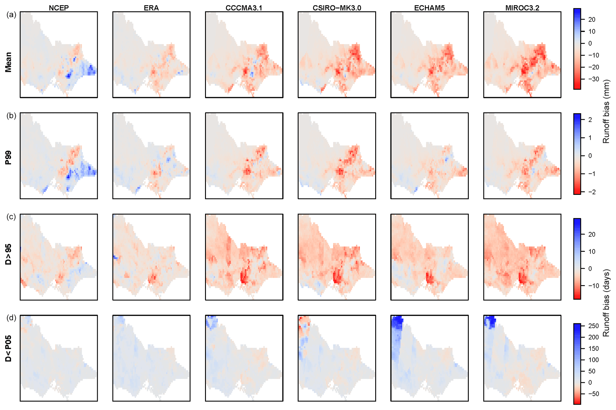
Figure 3Historical (1990–2009) runoff simulation bias (i.e. runoff using WRF-BC rainfall minus runoff using AWAP rainfall) for (a) mean annual runoff (mm), (b) daily 99th-percentile runoff (mm), (c) number of days exceeding AWAP 95th percentile and (d) number of days below AWAP 10th percentile. Columns (left to right) are using WRF-BC rainfall forced by two reanalyses (NNR and ERAI) and then four GCMs (CCCMA3.1, CSIRO-MK3.0, ECHAM5 and MIROC3.2).
Additionally, Potter et al. (2020) have shown that the QQM-BC approach does not correct for other particular rainfall characteristics. These include the underestimation of (i) wet–wet-day transition probabilities (i.e. frequency of consecutive wet days), (ii) multi-day rainfall accumulations and (iii) spatial correlation of rainfall events. Thus, despite WRF-BC slightly overestimating annual mean rainfall compared to AWAP (Fig. 2b), the underestimation of wet–wet-day transition probabilities and multi-day rainfall accumulations resulted in an underestimation of simulated runoff when compared to runoff simulated using observed (i.e. AWAP) rainfall inputs, as shown in Fig. 3. There was an underestimation of mean annual runoff, high flows (99th-percentile daily flow) and the number of high-flow days (days above 95th-percentile flow) in most cases (Fig. 3). The magnitude of the underestimations was larger for the GCM-forced runs compared to the reanalysis-forced runs, and (in contrast) NNR-based results for the south-east produced some overestimation biases. The magnitudes of these biases are compared to the magnitudes of their respective climate change signals (projected future minus historical) in the next section.
3.2 Projected future simulations
The influence that the bias correction (QQM-BC) has had on WRF rainfall change was assessed by comparing the WRF-BC change (BC future minus BC historical) to that obtained from empirically scaled (ES) change (i.e. from applying the raw-future-minus-raw-historical change to AWAP historical). The ES AWAP rainfall, scaled separately according to both WRF-raw (i) annual and (ii) seasonal rainfall changes, produced “annual ES change” and “seasonal ES change”, respectively.
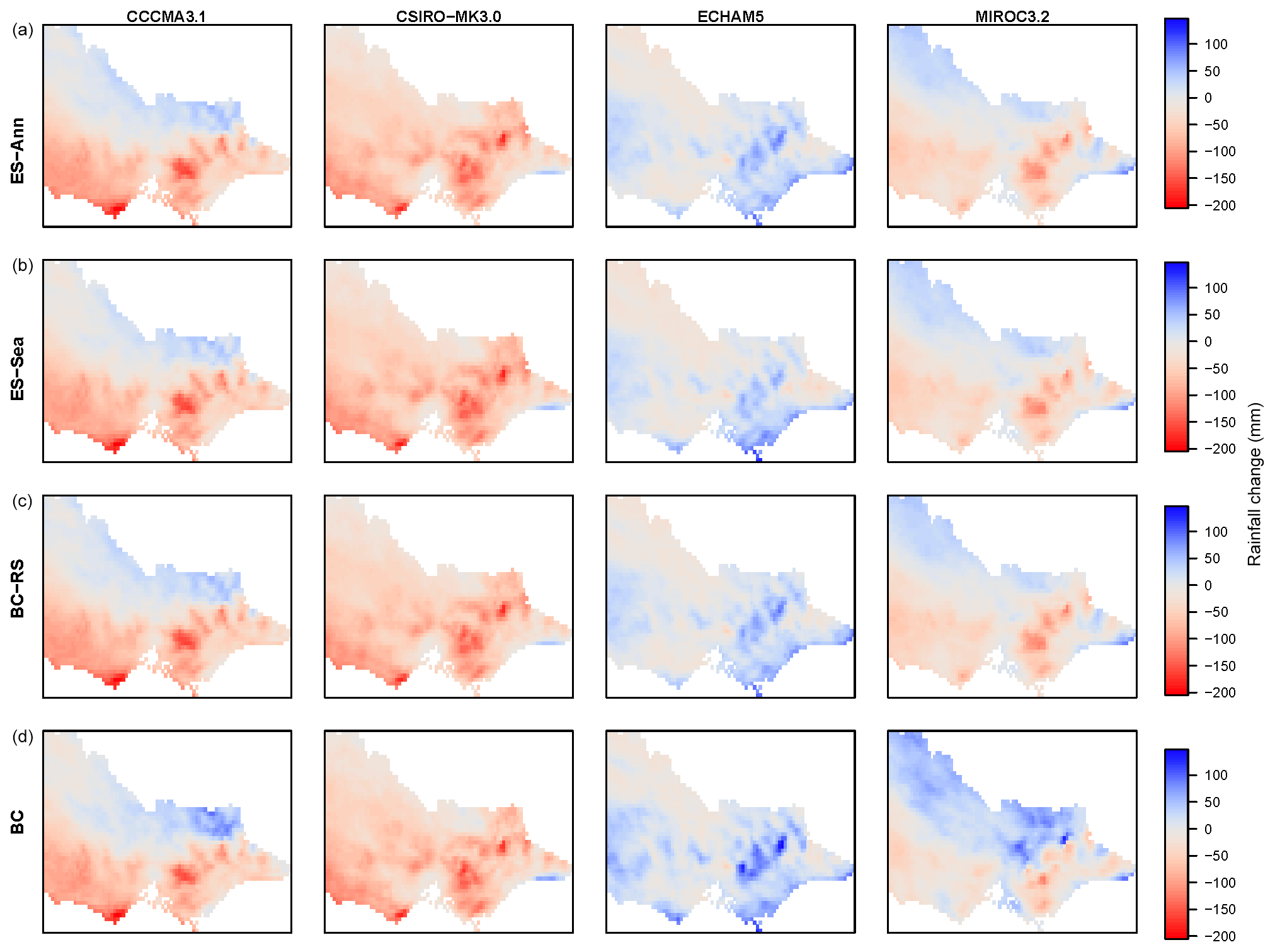
Figure 4Mean annual rainfall change (mm) for (a) empirical annual scaling, (b) empirical season scaling, (c) BC rescaled (according to ES seasonal then annual changes) and (d) BC. Columns (left to right) show CCCMA3.1, CSIRO-MK3.0, ECHAM5 and MIROC3.2.
Differences between the annual rainfall changes obtained from the annual ES (Fig. 4a) and seasonal ES (Fig. 4b) indicated differences between WRF and AWAP rainfall seasonality. For example, in the case of the ECHAM5-forced results there was a Victoria-average annual rainfall increase of 4.8 mm using seasonal ES compared to 9.6 mm using annual ES. Thus ECHAM5-forced WRF must have produced too much rain in one or more seasons, compared to AWAP seasonality, to result in this discrepancy between seasonal and annual ES changes. That is, if the proportion contributed by each season had been similar between ECHAM5-forced WRF and AWAP, then the seasonal and annual ES would have produced similar annual changes, as can be seen for the remaining three GCM-forced cases.
The WRF-BC future rainfall was also rescaled for comparison with ES results (rescaled twice, seasonally then annually) so as to match the WRF-raw annual rainfall change signal, as shown in Fig. 4c (i.e. the change signal in mean annual rainfall is the same in Fig. 4a, b and c). In general the WRF-BC rainfall changes (Fig. 4d) were wetter (or less dry) changes than both the WRF-BC rescaled and the ES changes (Fig. 4a, b and c). In the example of ECHAM5-forced results, the seasonal ES gave a 4.8 mm Victoria-average increase, whereas BC gave an increase of 16.7 mm, with the changes showing similar spatial patterns but with BC giving larger increases particularly over the high-altitude areas.
It was also possible for WRF-BC rainfall change to have a different change direction to that of the WRF-raw rainfall, as evident for MIROC3.2-forced results in the north-east Victorian Alps where the BC has a positive (i.e. wetter) change in contrast to the ES (i.e. WRF-raw) having a negative (i.e. drier) change. Hence there was a difference between the seasonal ES average decline of −14.9 mm and the corresponding BC increase of 8.6 mm. In contrast, the magnitudes and spatial patterns of BC and ES changes were much more similar to each other for the results from WRF CCCMA3.1 and CSIRO-Mk3.0-forced results (Fig. 4).
The impact of these BC and ES rainfall differences on their corresponding simulated runoff changes were assessed by comparing runoff simulations using four rainfall input variations, namely (a) ES-ann: AWAP rainfall scaled according to WRF-raw annual rainfall changes; (b) ES-seaann: AWAP rainfall scaled twice, firstly according to WRF-raw seasonal rainfall changes and then rescaled to match WRF-raw annual rainfall changes; (c) BC RS: the WRF-BC future rainfall scaled twice, firstly so as to match WRF-raw seasonal rainfall changes and then rescaled to match WRF-raw annual rainfall changes; and (d) BC: the WRF-BC rainfall. For (a) and (b) the runoff changes were the difference in simulated runoff using ES-future relative to AWAP-historical rainfall, whereas for (c) and (d) the runoff changes were the difference in simulated runoff using BC(-RS)-future relative to BC(-RS)-historical rainfall.
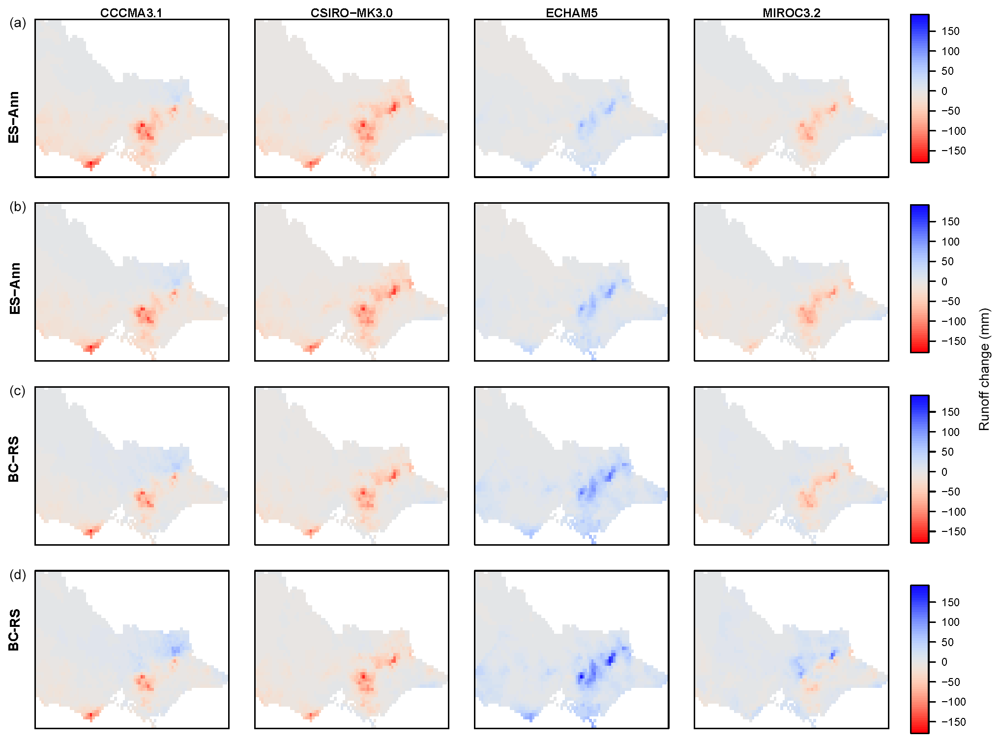
Figure 5Mean annual runoff change (mm, future minus historical) for (a) ES-ann, (b) ES-seaann, (c) BC RS and (d) BC. Columns (left to right) show CCCMA3.1, CSIRO-MK3.0, ECHAM5 and MIROC3.2.
Consistent with the rainfall change differences shown in Fig. 4, the mean annual runoff changes (Fig. 5) highlight that (i) BC produced greater runoff increases than ES for locations with increased runoff; (ii) BC correspondingly produced smaller runoff decreases than ES for locations with decreased runoff; and (iii) BC RS runoff change was drier than BC, albeit not as dry as the ES runoff changes. This is due to the combined effect of the remaining biases in BC RS rainfall (e.g. underestimation of wet–wet-day transitions and multi-day accumulations) and also rainfall characteristics that BC can change that are not accounted for by ES, such as changes to upper tails of daily rainfall distributions producing more intense extreme rainfall and sequencing of wet and dry days. That is, for wetter projections BC rainfall can have more frequent wet days and more intense rainfall extremes relative to ES, leading to larger BC runoff increases compared to ES (e.g. ECHAM5). The ability of BC rainfall to include changes in temporal characteristics is an important improvement over ES, given ES is constrained to reproducing the historical sequencing. Thus, for drier projections, such sequencing and upper-tail changes can mitigate the runoff decreases seen in the ES results (e.g. CCMA3.1 and CSIRO-Mk3.0). In some cases (e.g. MIROC3.2 for some areas) these factors have changed ES runoff decreases to BC runoff increases (Fig. 5). We address our confidence in such changes in the discussion section.
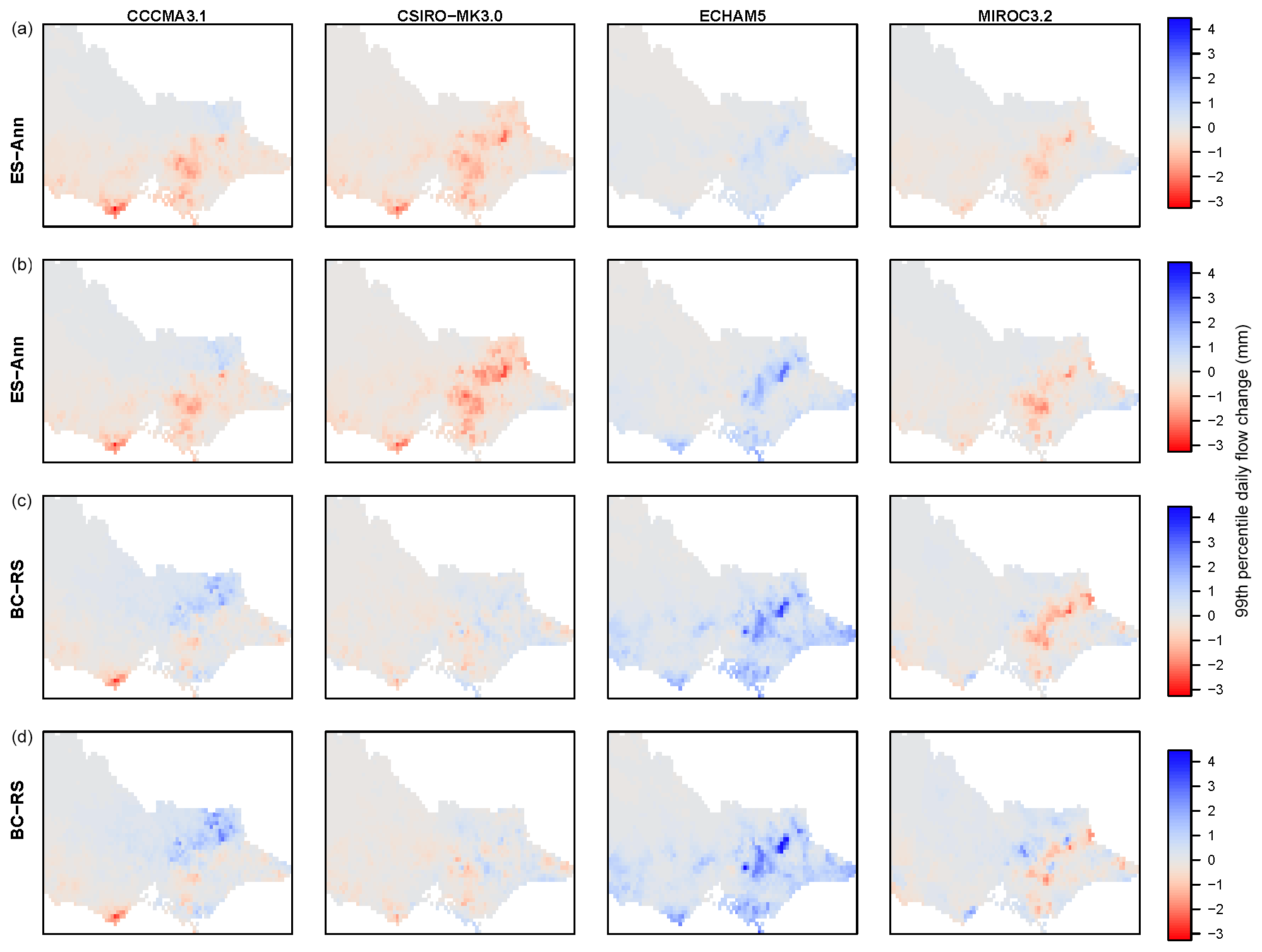
Figure 6Change in 99th-percentile daily flow (mm, future minus historical) for (a) ES-ann, (b) ES-seaann, (c) BC RS and (d) BC. Columns (left to right) show CCCMA3.1, CSIRO-MK3.0, ECHAM5 and MIROC3.2.
Correspondingly, the changes to 99th-percentile daily runoff (Fig. 6) show BC produced larger increases (or smaller decreases) than ES, and BC has changed the direction from decreases to increases for certain areas for all cases except ECHAM5-forced (which did not produce decreases). The BC RS changes are similar to (slightly less than) BC changes, indicating they are due to BC-derived changes in rainfall characteristics, such as changes to upper tails of rainfall distributions, and potentially changes in wet-day sequencing too, both of which influence high flows and were not accounted for by ES.
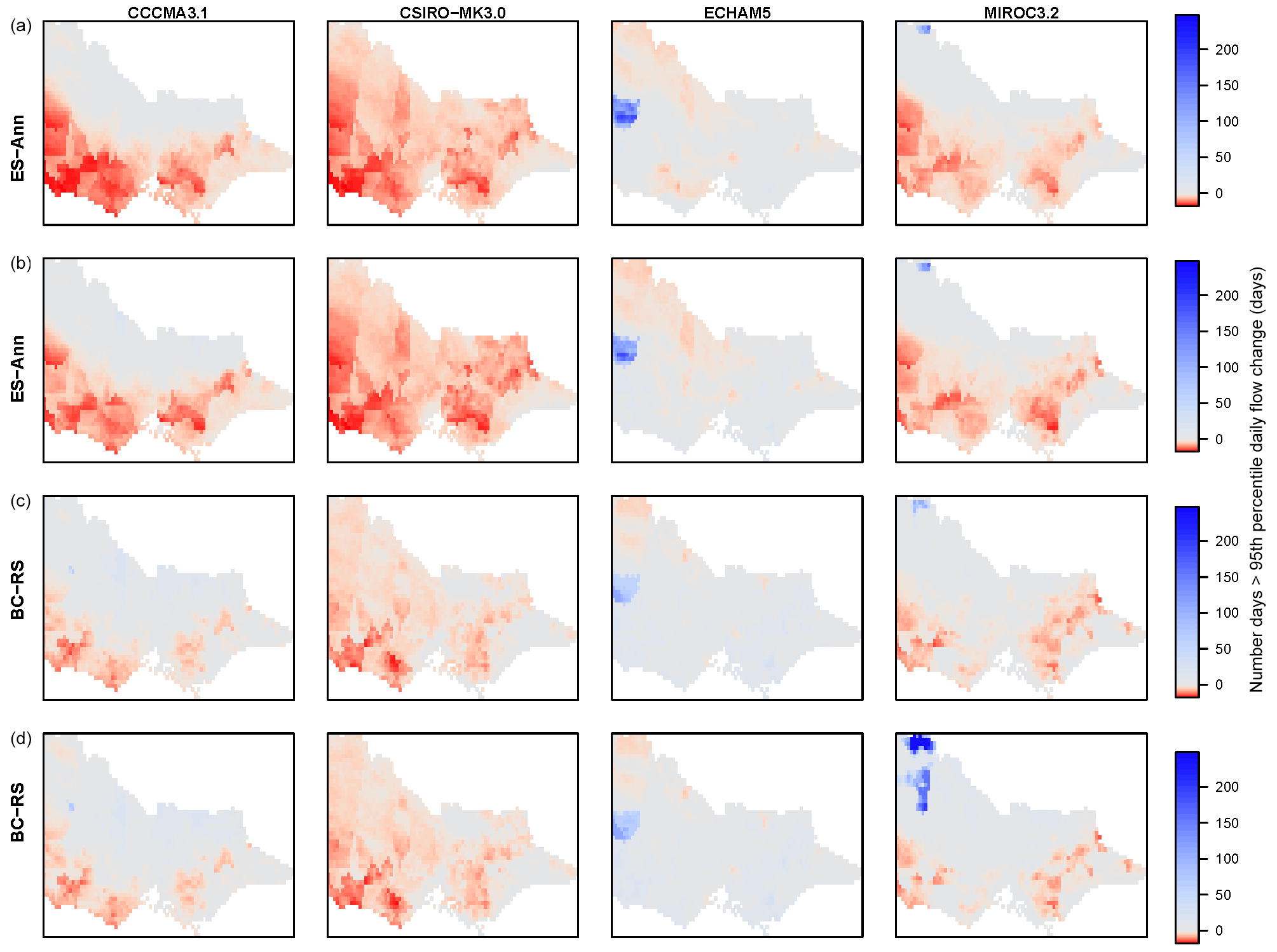
Figure 7Change in number of days exceeding historical 95th-percentile daily flow (future minus historical) for (a) ES-ann, (b) ES-seaann, (c) BC RS and (d) BC. Columns (left to right) show CCCMA3.1, CSIRO-MK3.0, ECHAM5 and MIROC3.2.
Changes to the frequency of high-flow days, i.e. number of days greater than the historical 95th-percentile daily flow, show larger increases and smaller decreases for BC compared to ES results (Fig. 7). BC RS results are changed compared to the BC results; however in most cases they remain closer to the original BC than ES results. One exception is MIROC3.2-forced results, where large BC increases in the NW are absent in BC RS.
3.3 Catchment-scale simulations
The change signal magnitudes are highly dependent on the driving GCM, with noticeable differences between lumped and distributed cases. Figure 8 shows a general pattern that, when there is a projected increase in runoff, in all cases the lumped results give larger increases than the distributed case. Likewise for projected decreases, there are greater decreases (i.e. more negative) for the lumped than for the distributed cases.
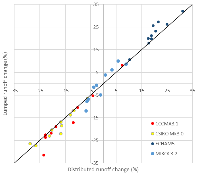
Figure 8Distributed versus lumped change (future period relative to current period) in mean annual runoff (%).
ECHAM5-forced results consistently simulate large runoff increases of at least +10 % and up to a +32 % increase. CSIRO-Mk3.0 consistently simulates the largest runoff decreases, of up to −29 %, and CCCMA3.1 simulates decreases (of up −32 %) for all catchments except for 403210. MIROC3.2 WRF-BC rainfall produces smaller changes, with a range from −12 % to +10 %.
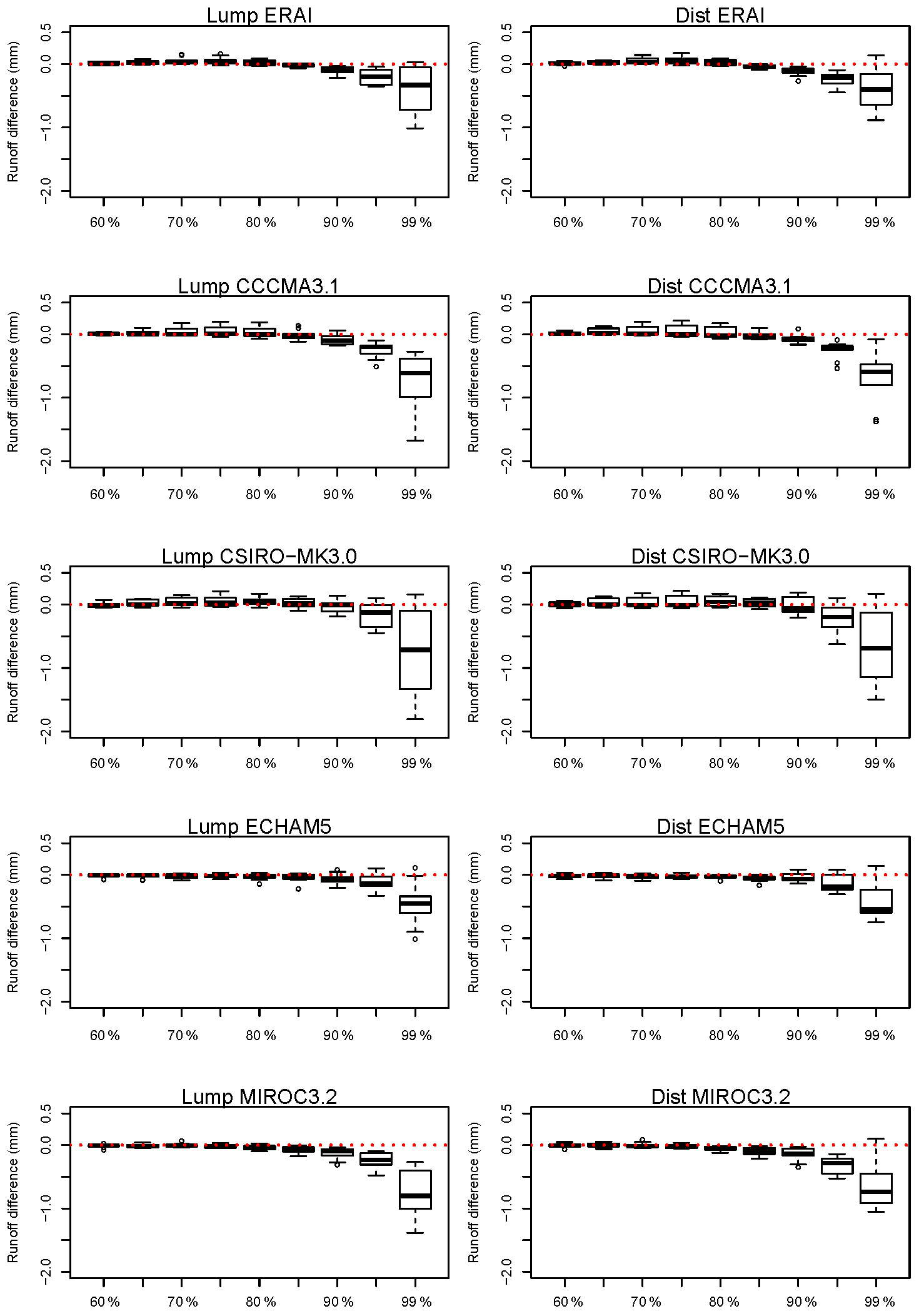
Figure 9Simulated historical-period runoff high-flow percentile bias (simulation using WRF-BC rainfall minus simulation using AWAP rainfall) of the 60th to 99th daily percentiles for lumped (left) and distributed (right) simulations. Negative values indicate WRF-BC-derived results are smaller than AWAP-derived results. Box plots show the range across the 10 catchments.
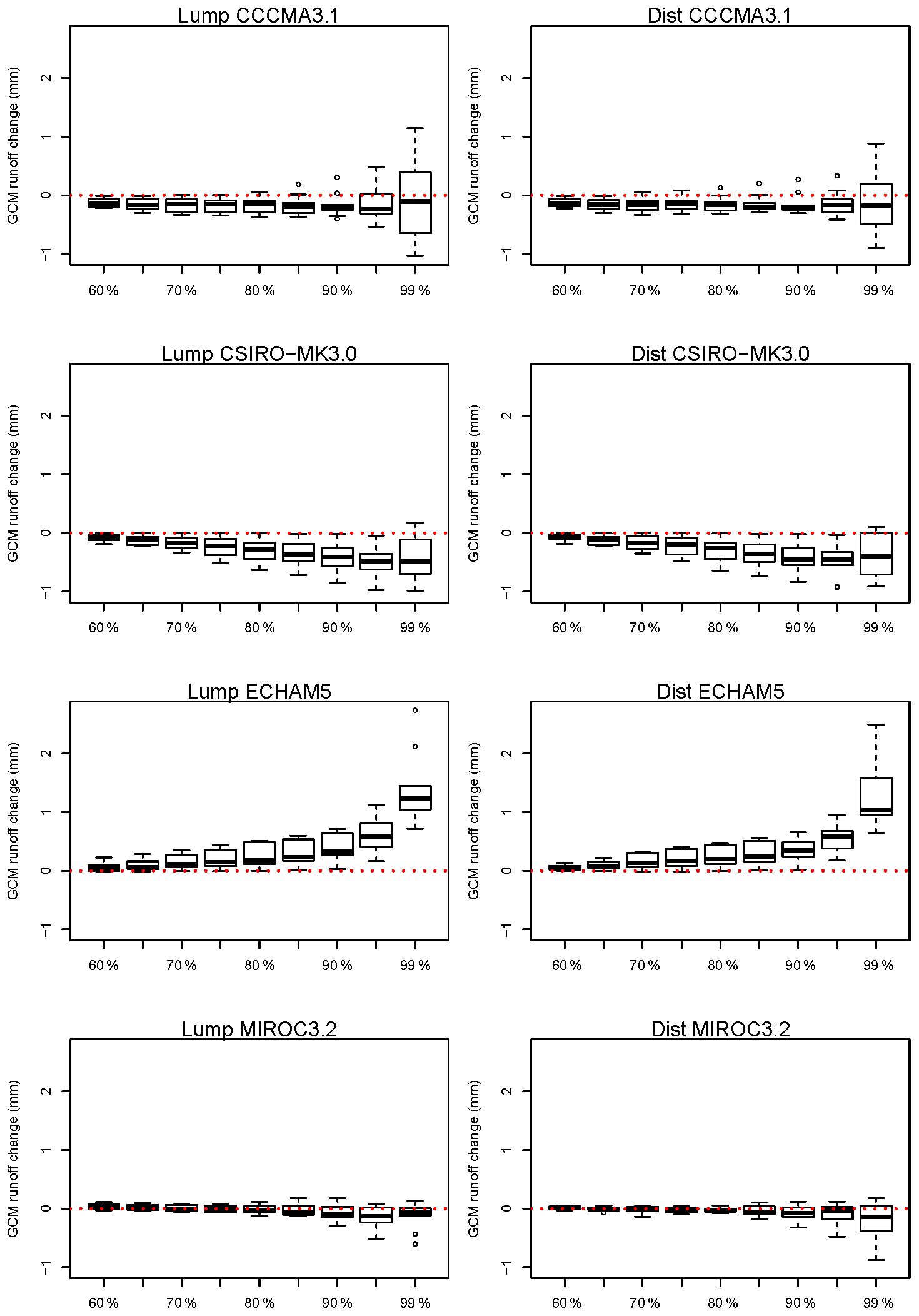
Figure 10Simulated climate change runoff high-flow percentile changes (future minus historical using WRF-BC rainfall) of the 60th to 99th daily percentiles for lumped (left) and distributed (right) simulations. Box plots show the range across the 10 catchments.
Given the historical runoff underestimation biases shown earlier (Fig. 3), we look at the bias in the simulation of high flows for the 10 catchments, for the distributed and lumped calibrations (Fig. 9). There are small differences for most of the percentiles shown, with a small underestimation of the 90th percentile becoming greater and more variable for the 99th percentile in all cases. The distributed 99th percentiles have slightly more underestimation than those for the lumped method for the reanalysis run, whereas for the four driving GCMs results the lumped results show slightly more underestimation than the distributed method. This underestimation of high flows (90th percentile and above) seen in most cases will result in underestimation of annual and monthly runoffs; the reasons for this underestimation are discussed later. The corresponding projected changes, shown in Fig. 10, show small decreases for CCCMA3.1 up to the 90th percentile and a large range from decreases to increases for the 95th and 99th percentiles. CSIRO-Mk3.0 presents a more consistent decrease with higher percentiles, with a larger range for the 99th, with at least one catchment experiencing an increase. ECHAM5-forced results presents the most consistent projected changes, with increases particularly for the 99th percentile. Relatively small changes, with mainly decreases for higher percentiles, are seen for MIROC3.2-forced results.
Potter et al. (2020) have shown that WRF-BC rainfall, while greatly improved over WRF-raw rainfall (Fig. 2), underestimates sequences of wet days, multi-day accumulations and daily rainfall spatial correlation. We show that these remaining biases result in the underestimation of simulated historical mean seasonal and annual runoff and high flows (Fig. 3). Whether these biases influence the magnitude of projected runoff change is the focus of the discussion presented here. Given that the characteristics of the WRF-raw rainfall changes are modified by QQM-BC (Fig. 4) and hence that the WRF-BC-rainfall-derived runoff changes are different (Fig. 5), there is a need to assess whether they are more or less realistic than the runoff changes produced simply by empirically scaling the historical rainfall series by the annual or seasonal change signal in the WRF-raw rainfall. Note that such a comparison does not rely on the ES-derived runoff changes being correct; i.e. we are not validating the BC-derived runoff changes against those from ES. We are merely attempting to determine whether BC runoff changes are more or less credible, in terms of the characteristics assessed herein.
There is an argument that, because the QQM-BC rainfall corrects distributional biases in the WRF-raw rainfall, the QQM-BC rainfall change signals are more realistic than those of the original WRF-raw rainfall; however Ehret et al. (2012) are cautious of this view, stating QQM-BC does not have physical justification. Hagemann et al. (2011), investigating hydrological changes globally, has noted that for some regions the magnitude of change in climate change signal due to bias correction can be greater than the magnitude of the signal itself, such that bias-correction uncertainty can be as large as climate model uncertainty. Several subsequent studies have investigated how bias correction modifies the rainfall climate change signal (Dosio et al., 2012; Ivanov et al., 2018; Mbaye et al., 2016; Potter et al., 2018; Sangelantoni et al., 2018; Themeßl et al., 2012). Themeßl et al. (2012) concluded that QQM-BC is likely to improve the reliability of projected changes if the climate model biases are related to the shape of the distribution, i.e. when RCM bias is magnitude-dependent. Dosio et al. (2012), investigating ENSEMBLES RCMs over Europe, noted that the RCMs had a tendency to overestimate extreme rainfall and hence the increases in P99 for their bias-corrected results were 2–3 times smaller than the original RCM increases. Mbaye et al. (2016) also found that BC reduced the changes in heavy-rainfall events. Ivanov et al. (2018) concluded that changes to the CCS due to bias correction are scientifically appropriate and therefore the BC CCS is more trustworthy than the raw CCS, due to the removal of model biases that adversely influence the original CCS. Given the large biases shown in Fig. 2, we did not have confidence in using WRF-raw rainfall as input to hydrological modelling; thus our findings implicitly agree with these previously published conclusions.
Regarding the BC-simulated hydrological changes for Victoria, comparison of the magnitude of BC mean runoff bias (in the historical period) (Fig. 3, top row) to BC mean runoff change (under projected climate change) (Fig. 5, bottom row) shows cases where the absolute value of Victorian area-average change is larger than the bias (CSIRO-Mk3.0-forced change: −8.7 mm, bias: −6.5 mm; ECHAM5-forced change: 15.4 mm, bias: −6.2 mm) and cases where the change is smaller than the bias (CCCMA3.1-forced change: −0.2 mm, bias: −5.5 mm; MIROC3.2-forced change: 5.23 mm, bias: −8.2 mm). However the range of bias is much smaller than the range of change, as evident by the scales on the respective plots (bias ranging from −30 to +20 mm; change ranging from −150 to +150 mm). Hence the bias is smaller and spatially consistent compared to the change signal.
The differences in runoff changes from empirically scaled rainfall (i.e. based on seasonal and/or annual changes in WRF-raw rainfall) and BC rainfall are shown in Figs. 5, 6 and 7 for annual mean runoff, daily 99th-percentile flow and the number of days above reference 95th-percentile flow, respectively. Comparing ES-ann- to ES-seaann-derived runoff changes shows similar mean runoff change (Fig. 5), with three GCM-forced cases very similar and ECHAM5-forced change larger for ES-seaann (6.2 mm) than for ES-ann (4.1 mm). For 99th percentile daily flow (Q99) (Fig. 6), the area-average values are similar; however larger changes (cases of both decreases and increases) are evident for certain regions.
Comparing ES-seaann- to BC-RS-derived runoff changes shows BC RS mean runoff change is wetter than ES-seaann in all four cases (Fig. 5). The ability of BC RS to include (through the BC, not the RS) changes to the upper tail of rainfall distributions and wet-day sequencing – in contrast to ES, which cannot – is likely to be the reason BC RS is wetter. Correspondingly, Q99 changes for BC RS are more positive than for ES-seaann (Fig. 6).
Comparing BC-RS- to BC-derived runoff changes shows BC mean runoff change to be wetter than BC RS, again in all four cases (Fig. 5). This supports the case that ES limitations are causing drier projections than BC, given that BC RS constrained to match ES-seaann changes is drier than BC. In three out of four cases the Q99 changes from BC are more positive than for those from BC RS (Fig. 6). Given Q99 is underestimated for historical BC (Fig. 3, second row), this suggests BC changes are more realistic than BC RS and hence also more realistic than ES changes in Q99; again this could be because BC can modify the upper tail of rainfall distributions and also wet-day sequencing.
Muerth et al. (2013) note that the more strongly biased a climate simulation is, the larger the effect of bias correction on the change signal of hydrological response. We see an example of this in the results from the MIROC3.2 GCM, which had the largest WRF-raw rainfall bias (Fig. 2) corresponding with the largest difference between ES and BC rainfall and runoff change (Figs. 4 and 5, respectively), including change of direction from ES runoff decreases to BC runoff increases in north-central and north-eastern regions. Confidence in such changes requires caution and relies on assuming the transferability of the BC from the historical to the future period (Velázquez et al., 2015). This assumption of transferability is a caveat on all BC but particularly impactful in this example.
The remaining BC rainfall biases add uncertainty to the magnitude of runoff changes, as rainfall that correctly reproduced wet-day sequencing and multi-day totals would potentially produce different runoff changes. If BC rainfall did not have the wet-to-wet-day transition and multi-day total underestimation biases, then projected increases could be greater and decreases lesser. Hence confidence in BC results is diminished because of these remaining rainfall biases. That is, while the BC rainfall change could be more realistic than WRF-raw and ES changes, for the reasons noted above, they would be more credible without the remaining biases in these rainfall characteristics.
We note that GR4J model performance for future climate conditions differing from the calibration period are an additional source of uncertainty (Stephens et al., 2019), but we do not assess such potential deficiencies here. We assume the bias of the model is constant for both the reference period and the projection period. Although it is worth exploring model performance under different climate conditions, the uncertainty from the discrepancy is assumed to be relatively small. This is because the model was calibrated for a long period covering different climate conditions to find robust parameters. At catchment scales, spatial correlation in WRF-raw and WRF-BC rainfall is underestimated and thus runoff is underestimated. This is an additional uncertainty and unaccounted source of bias in catchment runoff change, also leading to underestimation in projected runoff changes (Fig. 8). For historical-period simulations, the annual runoff has a longer and greater upper tail for the lumped simulations compared to the distributed cases. Correspondingly, the lumped upper quartile ranges are greater and the lower quartile ranges are smaller relative to distributed ones. Seasonally, for the low-flow summer and autumn seasons, the lumped flow has a larger range than distributed. For winter, lumped simulations produce greater median flows and upper tails. In spring, median and upper-tail differences are less pronounced, with smaller lower tails in the lumped simulations. Regarding the climate change signal, annually, lumped simulations tend to produce wetter changes than distributed simulations (an exception is the dry CSIRO-Mk3.0, which is slightly drier for lumped simulations. Seasonally, runoff changes are small (in absolute terms) for summer and autumn. Consistent dry projections are seen for spring, with lumped simulations slightly drier than distributed simulations in contrast to other seasons. For winter, lumped simulations are similar to distributed ones, with wetter projections having longer upper tails.
As shown in Figs. 9 and 10, for CSIRO-Mk3.0-forced results the combination of an underestimation of the highest daily flows for historical conditions and a projection for decreases in these high daily flows in the future means the runoff change may be overestimated (i.e. too large a projected decrease in runoff). For ECHAM5-forced results, which also underestimate the historical high flows, the projected increases may inherently underestimate the runoff increases.
Using WRF-BC rainfall from historical GCM-forced simulations to drive GR4J models produces underestimates of reference runoff. This underestimation is because the spell lengths of consecutive wet days are underestimated by WRF-BC rainfall, compared to observed rainfall, and hence the upper tail of the runoff distribution is underestimated.
For projected climate change impact on runoff, using WRF-raw rainfall would be unrealistic because the runoff overestimates for historical climate mean that any projected increase in rainfall will produce too large an increase in runoff and any decrease in rainfall will produce too small a decrease in runoff for these particular catchments. For the WRF-BC-rainfall-derived runoff changes, where historical runoff is underestimated, an increase in rainfall may underestimate the runoff increase and a decrease in rainfall may overestimate the runoff decrease. This study has attempted to understand and document some of these issues and impacts regarding how RCM BC influences hydrological simulations (Addor and Seibert, 2014), leading to the following conclusions:
-
There is a need for reporting of the caveats and influences that methodological choices have on projected hydrological changes derived from dynamically downscaled rainfall.
-
WRF-downscaled rainfall requires bias correction to be suitable for hydrological model input. QQM-BC can reproduce observed daily rainfall distributions for each grid cell; however QQM-BC rainfall underestimates wet-to-wet-day transition probabilities, multi-day totals and spatial correlation. These QQM-BC rainfall biases result in runoff biases, with runoff simulations underestimating mean seasonal, annual runoff and high flows.
-
WRF-raw rainfall changes are modified by QQM-BC, and thus runoff changes are modified also. Because the QQM-BC rainfall corrects distributional biases in WRF-raw rainfall, the QQM-BC rainfall change signals are plausibly more realistic than the changes of the WRF-raw rainfall.
-
Differences in projected future runoff changes from empirically scaled rainfall (i.e. based on WRF-raw rainfall changes) and QQM-BC rainfall are due to several factors, including limitations in ES not present in BC such as limited ability of ES to change multi-day rainfall distribution upper tails and sequencing. We conclude that BC runoff changes are more realistic than those from ES, with the caveat that the remaining BC rainfall biases due to underestimation of wet sequences, multi-day totals and spatial correlation need to be addressed to provide greater credibility for runoff projection.
-
The QQM-BC rainfall biases influence the magnitude of runoff changes, as discussed above; thus we conclude runoff increases may be underestimated and decreases overestimated. Additionally, as noted at catchment scales, spatial correlation in WRF-raw and hence QQM-BC rainfall is underestimated – an additional source of underestimation of projected runoff changes (Fig. 8).
Addor and Seibert (2014) discuss the need to better understand the underlying causes of these biases in climate models as well as a more systematic quantification of their impacts on hydrological response. Other recent studies have also questioned the application of BC without fully understanding the underlying reasons for the biases. Such studies have recommended “process-based” approaches to evaluate RCM simulation temporal and spatial realism, and thus credibility (Maraun et al., 2017; Maraun and Widmann, 2018). In future work we will assess multiple CMIP5-driven RCMs for their process performance in this region, with a view to developing rainfall bias-correction methods that can reduce biases in hydrological predictions. We will also continuing to develop and refine GR4J calibration and parameterisation methodologies to maximise suitability for hydrological predictions in a changing climate (Zheng et al., 2019).
We use AWAP gridded daily climate data provided by the Bureau of Meteorology, Commonwealth of Australia, available by request from climatedata@bom.gov.au. We use WRF simulations provided by the NSW and ACT Regional Climate Modelling (NARCliM) project's NSW Climate Data Portal https://climatedata.environment.nsw.gov.au/ (NSW Climate Data Portal, 2020).
The supplement related to this article is available online at: https://doi.org/10.5194/hess-24-2981-2020-supplement.
SPC conceived and designed the experiments and wrote the paper; FHSC contributed to the design, analysis and interpretation of results; NJP, HZ and GF performed experiments, analysed data and produced results; LZ contributed to the design and interpretation of results.
The authors declare that they have no conflict of interest.
We thank Jason Evans, Giovanni Di Virgilio and Fei Ji for providing WRF output and advice. Thanks also to James Bennett for helpful comments on an earlier draft and to the editor and referees for their constructive advice during the discussion and review process.
This research has been supported by the Victorian Department of Environment, Land, Water and Planning and CSIRO (Victorian Water and Climate Initiative).
This paper was edited by Nadav Peleg and reviewed by Eylon Eylon Shamir and one anonymous referee.
Addor, N. and Seibert, J.: Bias correction for hydrological impact studies – beyond the daily perspective, Hydrolog. Process., 28, 4823–4828, https://doi.org/10.1002/hyp.10238, 2014.
Andréassian, V., Oddos, A., Michel, C., Anctil, F., Perrin, C., and Loumagne, C.: Impact of spatial aggregation of inputs and parameters on the efficiency of rainfall-runoff models: A theoretical study using chimera watersheds, Water Resour. Res., 40, W05209, https://doi.org/10.1029/2003wr002854, 2004.
Casanueva, A., Kotlarski, S., Herrera, S., Fernández, J., Gutiérrez, J. M., Boberg, F., Colette, A., Christensen, O. B., Goergen, K., Jacob, D., Keuler, K., Nikulin, G., Teichmann, C., and Vautard, R.: Daily precipitation statistics in a EURO-CORDEX RCM ensemble: added value of raw and bias-corrected high-resolution simulations, Clim. Dynam., 47, 719–737, https://doi.org/10.1007/s00382-015-2865-x, 2016.
Chen, J., Brissette, F. P., Chaumont, D., and Braun, M.: Finding appropriate bias correction methods in downscaling precipitation for hydrologic impact studies over North America, Water Resour. Res., 49, 4187–4205, https://doi.org/10.1002/wrcr.20331, 2013.
Chiew, F. H. S., Teng, J., Vaze, J., Post, D. A., Perraud, J. M., Kirono, D. G. C., and Viney, N. R.: Estimating climate change impact on runoff across southeast Australia: Method, results, and implications of the modeling method, Water Resour. Res., 45, W10414, https://doi.org/10.1029/2008WR007338, 2009.
Chiew, F. H. S., Potter, N. J., Vaze, J., Petheram, C., Zhang, L., Teng, J., and Post, D. A.: Observed hydrologic non-stationarity in far south-eastern Australia: implications for modelling and prediction, Stochastic Environ. Res. Risk Assess., 28, 3–15, https://doi.org/10.1007/s00477-013-0755-5, 2014.
Chiew, F. H. S., Zheng, H., Potter, N. J., Ekström, M., Grose, M. R., Kirono, D. G. C., Zhang, L., and Vaze, J.: Future runoff projections for Australia and science challenges in producing next generation projections, 22nd International Congress on Modelling and Simulation, 3–8 December 2017, Hobart, Tasmania, Australia, 2017.
Chiew, F. H. S., Zheng, H., and Potter, N. J.: Rainfall-Runoff Modelling Considerations to Predict Streamflow Characteristics in Ungauged Catchments and under Climate Change, Water, 10, 1319, https://doi.org/10.3390/w10101319, 2018.
DELWP: Victoria's Climate Science Report 2019, available at: https://www.climatechange.vic.gov.au/__data/assets/pdf_file/0029/442964/Victorias-Climate-Science-Report-2019.pdf (last access: 2 June 2020), 2019.
Di Luca, A., Argüeso, D., Evans, J. P., de Elía, R., and Laprise, R.: Quantifying the overall added value of dynamical downscaling and the contribution from different spatial scales, J. Geophys. Res.-Atmos., 121, 1575–1590, https://doi.org/10.1002/2015JD024009, 2016.
Dosio, A., Paruolo, P., and Rojas, R.: Bias correction of the ENSEMBLES high resolution climate change projections for use by impact models: Analysis of the climate change signal, J. Geophys. Res.-Atmos., 117, D17110, https://doi.org/10.1029/2012JD017968, 2012.
Ehret, U., Zehe, E., Wulfmeyer, V., Warrach-Sagi, K., and Liebert, J.: HESS Opinions “Should we apply bias correction to global and regional climate model data?”, Hydrol. Earth Syst. Sci., 16, 3391–3404, https://doi.org/10.5194/hess-16-3391-2012, 2012.
Ekström, M., Grose, M. R., and Whetton, P. H.: An appraisal of downscaling methods used in climate change research, Wiley Interdisciplinary Reviews: Climate Change, 6, 301–319, https://doi.org/10.1002/wcc.339, 2015.
Evans, J. P., Ji, F., Lee, C., Smith, P., Argüeso, D., and Fita, L.: Design of a regional climate modelling projection ensemble experiment – NARCliM, Geosci. Model Dev., 7, 621–629, https://doi.org/10.5194/gmd-7-621-2014, 2014.
Evans, J. P., Argueso, D., Olson, R., and Di Luca, A.: Bias-corrected regional climate projections of extreme rainfall in south-east Australia, Theor. Appl. Climatol., 130, 1085–1098, https://doi.org/10.1007/s00704-016-1949-9, 2017.
Grose, M. R., Moise, A. F., Timbal, B., Katzfey, J. J., Ekström, M., and Whetton, P. H.: Climate projections for southern Australian cool-season rainfall: insights from a downscaling comparison, Clim. Res., 62, 251–265, 2015.
Gudmundsson, L., Bremnes, J. B., Haugen, J. E., and Engen-Skaugen, T.: Technical Note: Downscaling RCM precipitation to the station scale using statistical transformations – a comparison of methods, Hydrol. Earth Syst. Sci., 16, 3383–3390, https://doi.org/10.5194/hess-16-3383-2012, 2012.
Hagemann, S., Chen, C., Haerter, J. O., Heinke, J., Gerten, D., and Piani, C.: Impact of a Statistical Bias Correction on the Projected Hydrological Changes Obtained from Three GCMs and Two Hydrology Models, J. Hydrometeorol., 12, 556–578, https://doi.org/10.1175/2011JHM1336.1, 2011.
Hope, P., Timbal, B., Hendon, H., Ekström, M., and Potter, N.: A synthesis of findings from the Victorian Climate Initiative (VicCI), Bureau of Meteorology, Melbourne, Australia, 56 pp., 2017.
IPCC: Workshop Report of the Intergovernmental Panel on Climate Change Workshop on Regional Climate Projections and their Use in Impacts and Risk Analysis Studies, edited by: Stocker, T. F., Qin, D., Plattner, G.-K., and Tignor, M., IPCC Working Group I Technical Support Unit, University of Bern, Bern, Switzerland, 171 pp., 2015.
Ivanov, M. A. and Kotlarski, S.: Assessing distribution-based climate model bias correction methods over an alpine domain: added value and limitations, Int. J. Climatol., 37, 2633–2653, https://doi.org/10.1002/joc.4870, 2017.
Ivanov, M. A., Luterbacher, J., and Kotlarski, S.: Climate Model Biases and Modification of the Climate Change Signal by Intensity-Dependent Bias Correction, J. Climate, 31, 6591–6610, https://doi.org/10.1175/JCLI-D-17-0765.1, 2018.
Ji, F., Evans, J. P., Teng, J., Scorgie, Y., Argüeso, D., and Di Luca, A.: Evaluation of long-term precipitation and temperature Weather Research and Forecasting simulations for southeast Australia, Clim. Res., 67, 99–115, 2016.
Jones, D. A., Wang, W., and Fawcett, R.: High-quality spatial climate data-sets for Australia, Aust. Meteorol. Ocean., 58, 233–248, 2009.
Kiem, A. S. and Verdon-Kidd, D. C.: Towards understanding hydroclimatic change in Victoria, Australia – preliminary insights into the “Big Dry”, Hydrol. Earth Syst. Sci., 14, 433–445, https://doi.org/10.5194/hess-14-433-2010, 2010.
Lafon, T., Dadson, S., Buys, G., and Prudhomme, C.: Bias correction of daily precipitation simulated by a regional climate model: a comparison of methods, Int. J. Climatol., 33, 1367–1381, https://doi.org/10.1002/joc.3518, 2013.
Maraun, D.: Bias Correcting Climate Change Simulations – a Critical Review, Curr. Clim. Change Rep., 2, 211–220, https://doi.org/10.1007/s40641-016-0050-x, 2016.
Maraun, D. and Widmann, M.: Cross-validation of bias-corrected climate simulations is misleading, Hydrol. Earth Syst. Sci., 22, 4867–4873, https://doi.org/10.5194/hess-22-4867-2018, 2018.
Maraun, D., Wetterhall, F., Ireson, A. M., Chandler, R. E., Kendon, E. J., Widmann, M., Brienen, S., Rust, H. W., Sauter, T., Themeßl, M., Venema, V. K. C., Chun, K. P., Goodess, C. M., Jones, R. G., Onof, C., Vrac, M., and Thiele-Eich, I.: Precipitation downscaling under climate change: Recent developments to bridge the gap between dynamical models and the end user, Rev. Geophys., 48, RG3003, https://doi.org/10.1029/2009RG000314, 2010.
Maraun, D., Shepherd, T. G., Widmann, M., Zappa, G., Walton, D., Gutierrez, J. M., Hagemann, S., Richter, I., Soares, P. M. M., Hall, A., and Mearns, L. O.: Towards process-informed bias correction of climate change simulations, Nat. Clim. Change, 7, 664–773, https://doi.org/10.1038/nclimate3418, 2017.
Mbaye, M. L., Haensler, A., Hagemann, S., Gaye, A. T., Moseley, C., and Afouda, A.: Impact of statistical bias correction on the projected climate change signals of the regional climate model REMO over the Senegal River Basin, Int. J. Climatol., 36, 2035–2049, https://doi.org/10.1002/joc.4478, 2016.
Muerth, M. J., Gauvin St-Denis, B., Ricard, S., Velázquez, J. A., Schmid, J., Minville, M., Caya, D., Chaumont, D., Ludwig, R., and Turcotte, R.: On the need for bias correction in regional climate scenarios to assess climate change impacts on river runoff, Hydrol. Earth Syst. Sci., 17, 1189–1204, https://doi.org/10.5194/hess-17-1189-2013, 2013.
Nakicenovic, N., Alcamo, J., Davis, G., de Vries, B., Fenhann, J., Gaffin, S., Gregory, K., Griibler, A., Jung, T. Y., Kram, T., La Rovere, E. L., Michaelis, L., Mori, S., Morita, T., Pepper, W., Pitcher, H., Price, L., Riahi, K., Roehrl, A., Rogner, H.-H., Sankovski, A., Schlesinger, M., Shukla, P., Smith, S., Swart, R., van Rooijen, S., Victor, N., and Dadi, Z.: Special Report on Emissions Scenarios: A Special Report of Working Group III of the Intergovernmental Panel on Climate Change, edited by: Nakicenovic, N. and Swart, R., Cambridge University Press, Cambridge, UK, 599 pp., 2000.
NSW Climate Data Portal: Regional Climate Model (RCM) simulations performed as part of the NSW and ACT Regional Climate Modelling (NARCliM) project, available at: https://climatedata.environment.nsw.gov.au/, last access: 5 June 2020.
Olson, R., Evans, J. P., Di Luca, A., and Argüeso, D.: The NARCliM project: model agreement and significance of climate projections, Clim. Res., 69, 209–227, 2016.
Perrin, C., Michel, C., and Andréassian, V.: Improvement of a parsimonious model for streamflow simulation, J. Hydrol., 279, 275–289, https://doi.org/10.1016/S0022-1694(03)00225-7, 2003.
Peters, G. P., Andrew, R. M., Boden, T., Canadell, J. G., Ciais, P., Le Quéré, C., Marland, G., Raupach, M. R., and Wilson, C.: The challenge to keep global warming below 2 ∘C, Nat. Clim. Chang., 3, 4–6, https://doi.org/10.1038/nclimate1783, 2013.
Potter, N. J. and Chiew, F. H. S.: An investigation into changes in climate characteristics causing the recent very low runoff in the southern Murray-Darling Basin using rainfall-runoff models, Water Resour. Res., 47, W00G10, https://doi.org/10.1029/2010wr010333, 2011.
Potter, N. J., Chiew, F. H. S., Zheng, H., Ekström, M., and Zhang, L.: Hydroclimate projections for Victoria at 2040 and 2065, CSIRO, Australia, available at: https://publications.csiro.au/rpr/pub?pid=csiro:EP161427 (last access: 2 June 2020), 2016.
Potter, N. J., Ekström, M., Chiew, F. H. S., Zhang, L., and Fu, G.: Change-signal impacts in downscaled data and its influence on hydroclimate projections, J. Hydrol., 564, 12–25, https://doi.org/10.1016/j.jhydrol.2018.06.018, 2018.
Potter, N. J., Chiew, F. H. S., Charles, S. P., Fu, G., Zheng, H., and Zhang, L.: Bias in dynamically downscaled rainfall characteristics for hydroclimatic projections, Hydrol. Earth Syst. Sci., 24, 2963–2979, https://doi.org/10.5194/hess-24-2963-2020, 2020.
Rajczak, J., Kotlarski, S., and Schär, C.: Does Quantile Mapping of Simulated Precipitation Correct for Biases in Transition Probabilities and Spell Lengths?, J. Climate, 29, 1605–1615, https://doi.org/10.1175/JCLI-D-15-0162.1, 2016.
Rasmussen, S. H., Christensen, J. H., Drews, M., Gochis, D. J., and Refsgaard, J. C.: Spatial-Scale Characteristics of Precipitation Simulated by Regional Climate Models and the Implications for Hydrological Modeling, J. Hydrometeorol., 13, 1817–1835, https://doi.org/10.1175/jhm-d-12-07.1, 2012.
Räty, O., Räisänen, J., and Ylhäisi, J. S.: Evaluation of delta change and bias correction methods for future daily precipitation: intermodel cross-validation using ENSEMBLES simulations, Clim. Dynam., 42, 2287–2303, https://doi.org/10.1007/s00382-014-2130-8, 2014.
Rummukainen, M.: Added value in regional climate modeling, WIRES Clim. Change, 7, 145–159, https://doi.org/10.1002/wcc.378, 2016.
Sangelantoni, L., Russo, A., and Gennaretti, F.: Impact of bias correction and downscaling through quantile mapping on simulated climate change signal: a case study over Central Italy, Theor. Appl. Climatol., 135, 725–740, https://doi.org/10.1007/s00704-018-2406-8, 2018.
Stephens, C. M., Marshall, L. A., and Johnson, F. M.: Investigating strategies to improve hydrologic model performance in a changing climate, J. Hydrol., 579, 124219, https://doi.org/10.1016/j.jhydrol.2019.124219, 2019.
Switanek, M. B., Troch, P. A., Castro, C. L., Leuprecht, A., Chang, H.-I., Mukherjee, R., and Demaria, E. M. C.: Scaled distribution mapping: a bias correction method that preserves raw climate model projected changes, Hydrol. Earth Syst. Sci., 21, 2649–2666, https://doi.org/10.5194/hess-21-2649-2017, 2017.
Teng, J., Potter, N. J., Chiew, F. H. S., Zhang, L., Wang, B., Vaze, J., and Evans, J. P.: How does bias correction of regional climate model precipitation affect modelled runoff?, Hydrol. Earth Syst. Sci., 19, 711–728, https://doi.org/10.5194/hess-19-711-2015, 2015.
Teutschbein, C. and Seibert, J.: Bias correction of regional climate model simulations for hydrological climate-change impact studies: Review and evaluation of different methods, J. Hydrol., 456–457, 12–29, https://doi.org/10.1016/j.jhydrol.2012.05.052, 2012.
Teutschbein, C. and Seibert, J.: Is bias correction of regional climate model (RCM) simulations possible for non-stationary conditions?, Hydrol. Earth Syst. Sci., 17, 5061–5077, https://doi.org/10.5194/hess-17-5061-2013, 2013.
Themeßl, M. J., Gobiet, A., and Heinrich, G.: Empirical-statistical downscaling and error correction of regional climate models and its impact on the climate change signal, Climatic Change, 112, 449–468, https://doi.org/10.1007/s10584-011-0224-4, 2012.
Velázquez, J. A., Troin, M., Caya, D., and Brissette, F.: Evaluating the Time-Invariance Hypothesis of Climate Model Bias Correction: Implications for Hydrological Impact Studies, J. Hydrometeorol., 16, 2013–2026, https://doi.org/10.1175/JHM-D-14-0159.1, 2015.
Viney, N. R., Perraud, J., Vaze, J., Chiew, F. H. S., Post, D. A., and Yang, A.: The usefulness of bias constraints in model calibration for regionalisation to ungauged catchments, In Proceedings of the MODSIM2009 International Congress on Modelling and Simulation, 13–17 July 2009, Cairns, Australia, 3421–3427, 2009.
Woldemeskel, F. M., Sharma, A., Sivakumar, B., and Mehrotra, R.: Quantification of precipitation and temperature uncertainties simulated by CMIP3 and CMIP5 models, J. Geophys. Res.-Atmos., 121, 3–17, https://doi.org/10.1002/2015jd023719, 2016.
Zheng, H., Chiew, F. H. S., Potter, N. J., and Kirono, D. G. C.: Projections of water futures for Australia: an update, in: MODSIM2019, 23rd International Congress on Modelling and Simulation. Modelling and Simulation Society of Australia and New Zealand, 1–6 December 2019, Canberra, Australia, edited by: Elsawah, S., ISBN 978-0-9758400-9-2, 1000–1006, https://doi.org/10.36334/modsim.2019.K7.zhengH, 2019.