the Creative Commons Attribution 4.0 License.
the Creative Commons Attribution 4.0 License.
 | 10 Jun 2020
Disentangling temporal and population variability in plant root water uptake from stable isotopic analysis: when rooting depth matters in labeling studies
Valentin Couvreur
Félicien Meunier
Thierry Bariac
Philippe Biron
Jean-Louis Durand
Patricia Richard
Mathieu Javaux
Isotopic labeling techniques have the potential to minimize the uncertainty of plant root water uptake (RWU) profiles estimated using multisource (statistical) modeling by artificially enhancing the soil water isotopic gradient. On the other end of the modeling continuum, physical models can account for hydrodynamic constraints to RWU if simultaneous soil and plant water status data are available.
In this study, a population of tall fescue (Festuca arundinacea cv. Soni) was grown in amacro-rhizotron and monitored for a 34 h long period following the oxygen stable isotopic (18O) labeling of deep soil water. Aboveground variables included tiller and leaf water oxygen isotopic compositions (δtiller and δleaf, respectively) as well as leaf water potential (ψleaf), relative humidity, and transpiration rate. Belowground profiles of root length density (RLD), soil water content, and isotopic composition were also sampled. While there were strong correlations between hydraulic variables as well as between isotopic variables, the experimental results underlined the partial disconnect between the temporal dynamics of hydraulic and isotopic variables.
In order to dissect the problem, we reproduced both types of observations with a one-dimensional physical model of water flow in the soil–plant domain for 60 different realistic RLD profiles. While simulated ψleaf followed clear temporal variations with small differences across plants, as if they were “onboard the same roller coaster”, simulated δtiller values within the plant population were rather heterogeneous (“swarm-like”) with relatively little temporal variation and a strong sensitivity to rooting depth. Thus, the physical model explained the discrepancy between isotopic and hydraulic observations: the variability captured by δtiller reflected the spatial heterogeneity in the rooting depth in the soil region influenced by the labeling and may not correlate with the temporal dynamics of ψleaf. In other words, ψleaf varied in time with transpiration rate, while δtiller varied across plants with rooting depth.
For comparison purposes, a Bayesian statistical model was also used to simulate RWU. While it predicted relatively similar cumulative RWU profiles, the physical model could differentiate the spatial from the temporal dynamics of the isotopic composition. An important difference between the two types of RWU models was the ability of the physical model to simulate the occurrence of hydraulic lift in order to explain concomitant increases in the soil water content and the isotopic composition observed overnight above the soil labeling region.


Since the seminal work of Washburn and Smith (1934) where it was first reported that willow trees did not fractionate hydrogen stable isotopes in a hydroponic water solution during root water uptake (RWU), water stable isotopologues (1H2H16O and ) have been used as indicators for plant water sources in soils. In their review, Rothfuss and Javaux (2017) reported on no less than 40 publications between 2015 and 2016 in which RWU was retrieved from stable isotopic measurements. Novel measuring techniques (e.g., cavity ring-down spectroscopy, CRDS, and off-axis integrated cavity output spectroscopy, ICOS) that provide methods for fast and cost-effective water stable isotopic analyses certainly enable and emulate current research in that field. Water stable isotopologues are no longer powerful tracers waiting for technological developments (Yakir and Sternberg, 2000) but are on the verge of being used to their full potential to address eco-hydrological research questions and identify processes in the soil–plant–atmosphere continuum (Werner et al., 2012; Dubbert and Werner, 2019; Sprenger et al., 2016).
The isotopic determination of RWU profiles is based on the principle that the isotopic composition of xylem water at the outlet of the root system (i.e., in the first aerial and non-transpiring node of the plant) equals the sum of the product between the soil water isotopic composition and the relative contribution to RWU across plant water sources. Results only show reasonable precision when (i) the soil water isotopic composition depth gradient is strong and monotonic (which avoids issues of identifiability) and (ii) the temporal dynamics of RWU and the soil water isotopic composition are relatively low. Condition (i) is mostly fulfilled at the surface of the soil, whereas the soil water isotopic composition gradients usually become lower or nonexistent with increasing depth (due to the isotopic influence of the groundwater table and increasing dispersion with depth). As illustrated by Oerter and Bowen (2019), the lateral variability of the soil water isotopic composition profiles can become significant in the field and could have great implications for the representability and meaningfulness of isotopic-derived estimates of RWU profiles. Condition (ii) is often neglected, but it is required due to the instantaneous nature of the sap flow samples.
To overcome these limitations, labeling pulses have been increasingly used in recent works to artificially alter the natural isotopic gradients (e.g., Beyer et al., 2016, 2018; Grossiord et al., 2014; Jesch et al., 2018; Volkmann et al., 2016b). However, precise characterization of the artificial spatial (i.e., lateral and vertical) and temporal distributions of the soil water isotopic composition (driven by factors such as soil isotopic water flow) is crucial. The punctual assessments of the isotopic composition profiles following destructive sampling in the field and the subsequent extraction of water in the laboratory might not be spatially or temporally representative and can lead to erroneous estimates of RWU profiles (Orlowski et al., 2018, 2016).
The vast majority of isotopic studies use statistical (e.g., Bayesian) modeling to retrieve the RWU profile solely from the isotopic composition of water extracted in the soil and the shoot (Rothfuss and Javaux, 2017). However, when data on soil and plant water status are available, hydraulic modeling tools can also be used to connect different data types in a process-based manner and estimate root water uptake profiles (Passot et al., 2019). Some of the most simplistic models use one-dimensional relative root distribution and plant-scale hydraulic parameters (Sulis et al., 2019), whereas the most complex models rely on root architectures and root segment permeabilities (Meunier et al., 2017c). Only a handful of studies have coupled isotopic measurements in plant tissues and soil material with models describing RWU in a mechanistic manner. For instance, Meunier et al. (2017a) could both locate and quantify the volume of redistributed water by Lolium multiflorum by labeling of the soil with 18O-enriched water under controlled conditions.
Building on the work of Meunier et al. (2017a), the objectives of the present study were (i) to model the temporal dynamics of the isotopic composition of the RWU of a population of Festuca arundinacea cv. Soni (tall fescue) in a physically based manner (i.e., by accounting for soil, plant, and environmental factors) during a semi-controlled experiment following the isotopic labeling of deep soil water, (ii) to investigate the implication of the model-to-data fit quality in terms of the meaningfulness of the isotopic information to reconstruct RWU profiles, and (iii) to confront the simulated root water uptake profiles with estimations obtained on the basis of isotopic information alone (i.e., provided by a Bayesian mixing model).
Our experiment consisted of supplying labeled water to a macro-rhizotron in which tall fescue was grown. Data on the soil and plant oxygen stable isotopic composition and hydraulic status were monitored for 34 h. In the following, the oxygen isotopic composition of water will be expressed in per mil (‰) on the “delta” (δ18O) scale with respect to the international water standard V-SMOW (Vienna Standard Mean Ocean Water; Gonfiantini, 1978).
2.1 Rhizotron experimental setup
The macro-rhizotron (which had the following dimensions: 1.6 m ×1.0 m ×0.2 m; see picture in Appendix A) was placed inside a glasshouse (INRA, Lusignan, France), where it was continuously weighed (KE1500, Mettler-Toledo, resolution of 20 g) to monitor water effluxes (i.e., bare soil evaporation or evapotranspiration). Underneath the soil compartment and in contact with it, a water reservoir (height of 0.1 m) that was filled with gravel acted as the water table and allowed the supply of water to the rhizotron. The rhizotron was equipped with two sets of CS616 time domain reflectometer (TDR) profiles (Campbell Scientific, USA) with 30 cm long probe rods positioned at six depths (−0.05, −0.10, −0.30, −0.60, −1.05, and −1.30 m) and one profile of tensiometers (SMS 2000, SDEC-France) located at four depths (−0.05, −0.10, −0.30, and −0.60 m) in order to monitor the evolution of the soil water volumetric content (θ, in m3 m−3) and matric potential (ψsoil, in MPa). Finally, relative humidity (RH, %) was recorded above the vegetation with one humidity and temperature probe (HMP45D, Vaisala, Finland). The transparent polycarbonate sides (front and back) allowed for daily observations of the root maximal depth. The experimental setup allowed for the precise control of the amount and δ18O composition of soil input water. Another important feature was the soil depth (i.e., 1.60 m), which minimized the influence of the water table on superficial layers' water content and δ18O.
2.2 Soil properties and installation
The soil substrate originates from an agricultural field that is part of the Observatory of Environment Research (ORE), INRA, Lusignan, France (0∘60 W, 46∘250 N) which is classified as Dystric Cambisol (with a particle size distribution of 15 % sand, 65 % silt, and 20% clay). Prior to installation in the rhizotron, the substrate was sieved at 2 mm and dried in an air oven at 110 ∘C for 48 h to remove most of the residual water. A total of 450 kg of soil was filled into the rhizotron in 0.10 m increments and compacted in order to reach a dry bulk density value of ρb=1420 kg m−3. The closed-form soil water retention curve of van Genuchten (1980) was derived in a previous study by Meunier et al. (2017a) from synchronous measurements of soil water content and matric potential from the saturated to the residual water content (see Appendix B for its hydraulic parameters). It was used to compute the soil water matric potential (ψsoil, in MPa) on the basis of volumetric water content data during the present experiment.
2.3 Experimental protocol
After installation, the soil was gradually flooded with local water ( ‰) from the bottom reservoir up to the top of the profile for a period of 3 d in order to reduce the initial lateral and vertical heterogeneities in water content and δ18O as much as possible. The tall fescue (Festuca arundinacea cv. Soni) was sown at a seeding density of 3.6 g m−2 (which, for the rhizotron surface area of 0.2 m2, corresponded to roughly 300 plants) when the soil water content reached 0.25 m3 m−3 (corresponding to pF 2.3) at −0.05 m, as measured by the soil water sensors, and emerged 12 d later. During a period of 165 d following seeding, the tall fescue cover was exclusively watered from the reservoir with local water in order to (i) keep the soil bottom layer (< −1.3 m) close to water saturation and (ii) not disrupt the natural soil water δ18O profile.
A total of 166 d after seeding (DaS 166) the following conditions were fulfilled: (i) there was a strong soil water content gradient between the soil deep [−1.5 m, −1.0 m] and superficial [−0.3 m, 0 m] layers, and (ii) the tall fescue roots had reached a depth of −1.5 m (observed through the polycarbonate transparent sides). That same day at 17:00 LT, the reservoir's water was labeled and its δ18O was measured at +470 ‰. Soil was sampled before (DaS 166 at 15:45 LT) and after labeling on DaS 167 at 07:00 LT, DaS 167 at 17:00 LT, and DaS 168 at 05:00 LT, using a 2 cm diameter auger through the transparent polycarbonate side of the rhizotron on four occasions from the surface down to −1.3 m, for the determination of the soil gravimetric water content (θgrav, in kg kg−1) and the oxygen stable isotopic composition (δsoil, in ‰). The gravimetric water content was then converted to the volumetric water content (, in m3 m−3, where ρb is the bulk soil density and ρw is the water density). The hypothesis of a constant value for ρb across the reconstructed soil profile was further validated from the quality of the linear fit (a coefficient of determination, R2, of 1.0) between the θ values measured by the sensors at the six available depths (−0.05, −0.10, −0.30, −0.60, −1.05, and −1.30 m) and those computed from θgrav.
On 40 occasions during a 34 h long period, three whole plants were sampled from the vegetation (i.e., 120 plants were sampled in total from the cover). Each plant's tiller and leaves were pooled into two separate vials. Dead material as well as the oldest living leaf around each tiller were removed so as not to contaminate tiller samples with transpiring material (Durand et al., 2007). In addition, air water vapor was collected from the ambient atmosphere surrounding the rhizotron. The air was run at a flow rate of 1.5 L min−1 through two glass cold traps in series immersed in a mixture of dry ice and pure ethanol at −80 ∘C. Water from the plant (i.e., tillers and leaves) and soil samples was extracted by vacuum distillation for 14 to 16 h depending on the sample mass (e.g., ranging from 18 to 28 g for soil) at temperatures of 60 and 90 ∘C, respectively. The residual water vapor pressure at the end of each successful extraction procedure invariably reached 10−1 mbar. The oxygen isotopic compositions of tiller, leaf, and soil water (i.e., δtiller, δleaf, and δsoil) and that of atmospheric water vapor (δatm) were measured with an isotope-ratio mass spectrometer (ISOPREP-18, Optima, Fison, Great-Britain, precision accuracy of 0.15 ‰). Finally, the leaf water potential (ψleaf, in MPa) was monitored with a pressure chamber on two leaves per sampled plant, and the evapotranspiration rate (in m d−1) was derived from the changes in the mass of the rhizotron at the same temporal scale as plant sampling.
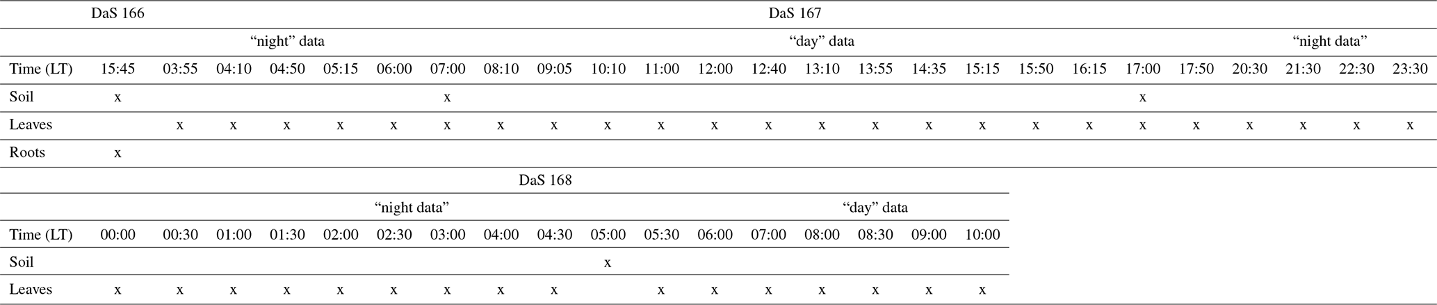
Root biomass was determined from the horizontal sampling of soil between the polycarbonate sides using a 2 cm diameter auger at soil depths of −0.02, −0.08, −0.10, −0.40, −0.55, −0.70, −0.90, −1.10, and −1.30 m. Each depth was sampled one to three times. Each soil core was washed of soil particles, and the roots were collected over a 0.2 mm mesh filter and dried at 60 ∘C for 48 h. Finally, the root length density (RLD, in meters of root per cubic meter of soil, m m−3) distribution was determined from the root dry mass using the specific root length of 95 m g−1 determined by Gonzalez-Dugo et al. (2005), which is explicitly for tall fescue. The reader is referred to Appendix C for an overview of the type and timing of the different destructive measurements during the intensive sampling period.
2.4 Modeling of RWU and δtiller
The experimental setup included about 300 tall fescue plants. In order to limit the computational requirement in the inverse modeling loop, we only generated 60 virtual root systems whose rooting depths ranged from a depth of −1.30 to −1.60 m (based on our own observations and those in the literature, e.g., Schulze et al., 1996; Fan et al., 2016) with the root architecture simulator CRootBox (Schnepf et al., 2018), so that the simulated RLD matched observations (Fig. 1a). In order to reach a total number of virtual plants representative of the number of plants in the experimental setup, each root system was replicated five times, forming a “group”. Each group was assumed to occupy 1/60 of the total horizontal area and was considered to be a “big root” hydraulic network (five identical plants per “big root”) with equivalent radial and axial hydraulic conductances (which neglects architectural aspects but accounts for each group's respective root length density profile).
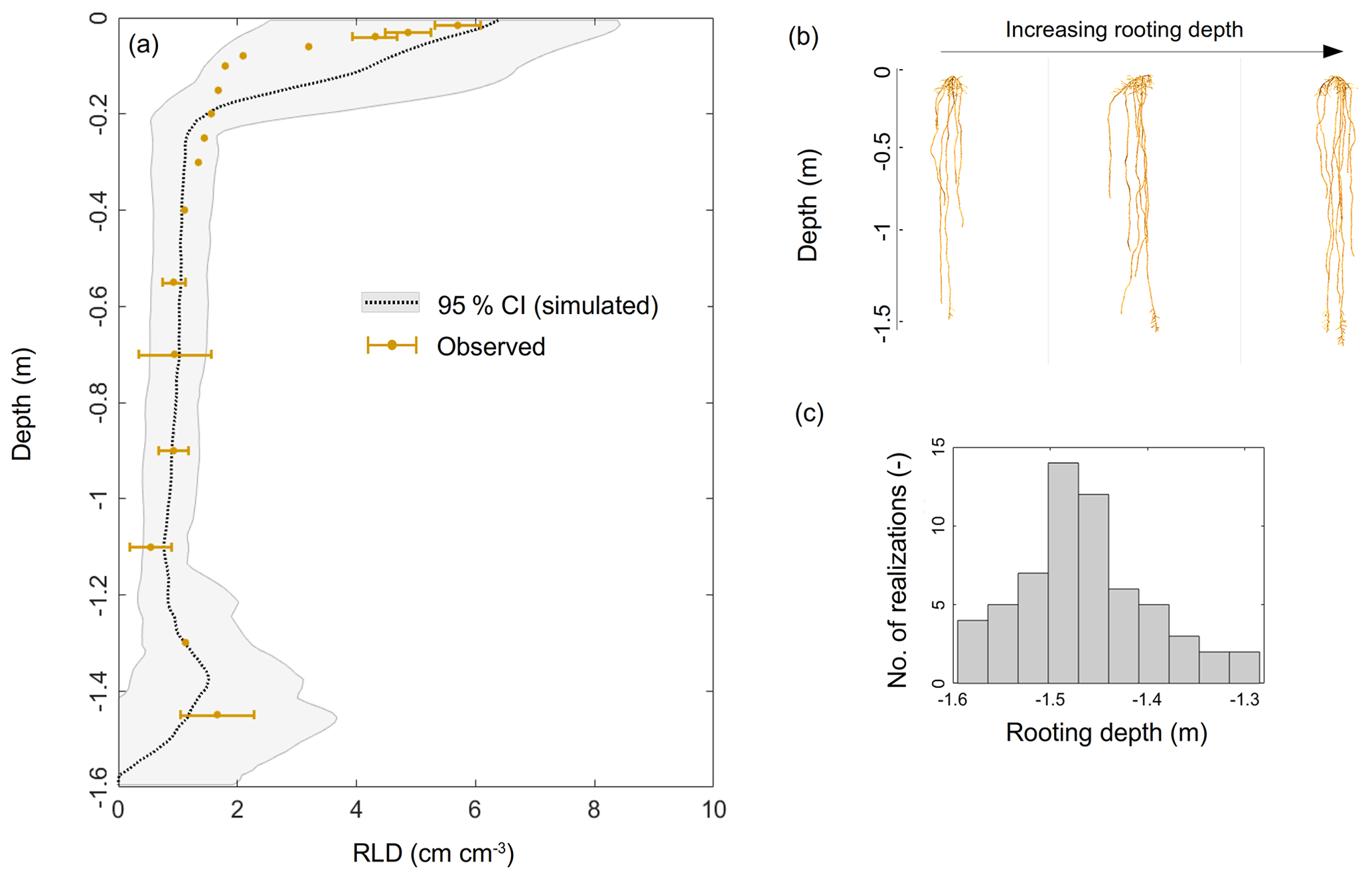
Figure 1(a) Simulated (gray shading) and observed (brown dots) root length density profiles. Panels (b) and (c) illustrate the variability in the modeled root system architectures and rooting depths, respectively.
The radial soil–root conductance between the bulk soil and each group's (i) root surfaces in soil layer j (Kradial,j, m3 MPa−1 d−1), as derived by Meunier et al. (2017a), was assumed to be variable in time (t):
Here, rroot (m) is the root radius, (m) is the root length of plants of group i in soil layer j, Lpr (m MPa−1 d−1) is the root radial hydraulic conductivity, ksoil,j (m2 MPa−1 d−1) is the soil hydraulic conductivity in layer j, and Bj (dimensionless) is a geometrical factor simplifying the horizontal dimensions into radial domains between the bulk soil and root surfaces, as given by Schroeder et al. (2009):
where ρ (dimensionless) represents the ratio of the distance between roots and the root averaged diameter. It can be deduced from the observed root length density (RLDj, m m−3) as follows:
The following soil hydraulic conductivity function of Mualem (1976) and van Genuchten (1980) was used:
where ksat (m2 MPa−1 d−1), m (dimensionless), and λ (dimensionless) are soil hydraulic parameters (with ), and Se,j, the relative water content (dimensionless), is computed from the saturated (θsat, m3 m−3) and residual (θres, m3 m−3) water contents as
Unlike the geometrical parameter B, which defines a domain geometry between the bulk soil and roots of the overall population, the lroot term is group specific (i) and uses the simulated root length density profiles over an area corresponding to 1/60 of the total setup horizontal area:
where ΔZ (m) and Asoil (m2) are the soil layer thickness and horizontal surface area, respectively.
To finalize the connection between root xylem and shoot, axial conductances per root system group (Kaxial, m3 MPa−1 d−1) were calculated as equivalent “big root” specific axial conductance per root system group (kaxial, m4 MPa−1 d−1, to be optimized by inverse modeling) as follows:
At each time step, both the total soil–root system conductance (Ksoil–root, m3 MPa−1 d−1) and the standard sink distribution (SSF, dimensionless, summing to 1), were calculated from Kradial and Kaxial, using the algorithm of Meunier et al. (2017b). The variable SSF is the relative distribution of water uptake in each soil layer under vertically homogeneous soil water potential conditions (Couvreur et al., 2012), and Ksoil–root represents the water flow per unit water potential difference between the SSF-averaged bulk soil water potential and the “big leaf” (assuming a negligible stem hydraulic resistance; Steudle and Peterson, 1998).
Adding soil hydraulic conductance to the one-dimensional hydraulic model of Couvreur et al. (2014) yields the following solutions for the leaf water potential (ψleaf, MPa) and water sink terms (S, d−1) whose formulation approaches that of Nimah and Hanks (1973):
where 1/60 of the overall transpiration rate (T, m d−1) is allocated to each group, and ψsoil,j (Mpa) is the soil water potential in soil layer j.
where, due to large axial conductances, Ksoil–root was assumed to control the compensatory RWU which arises from a heterogeneously distributed soil water potential (Couvreur et al., 2012).
Finally, the tiller water oxygen isotopic composition (δtiller) was calculated as the average of the local soil water oxygen isotopic compositions (δsoil) weighted by the relative distribution of positive water uptakes (i.e., not accounting for δsoil at locations where water is exuded by the root), assuming a perfect mixture of water inside the root system (Meunier et al., 2017a):
As in the experiment, δtiller from three plants were randomly pooled at each observation time. A total of 100 pools of three plants (possibly including several plants of the same group) were randomly selected in order to obtain the pooled simulated δtiller by arithmetic averaging.
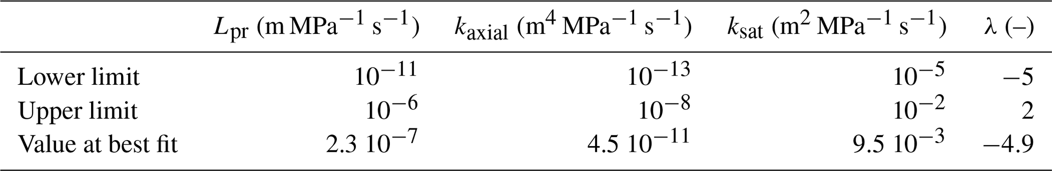
The unknown parameters of the soil–root hydraulic model, i.e., the root radial conductivity (Lpr), the root axial conductance (kaxial), the soil saturated hydraulic conductivity (ksat), and the soil tortuosity factor (λ), were finally determined by inverse modeling. For details on the procedure, the reader is referred to Appendix D.
In order to evaluate the robustness of the hydraulic model predictions (parameterized solely based on the reproduction of shoot observations in the inverse modeling scheme) from independent perspectives, we also compared predictions and measurements over four quantitative “soil–root domain” criteria: (i) the depth at which the transition between nighttime water uptake and exudation (Si,j < 0, i.e., the release of water from the root to soil) takes place, (ii) the quantities of exuded water and the overnight increase in the soil water content, (iii) the enrichment of labeled water at the depth where the water content increase is observed overnight, and (iv) the order of magnitude of the optimal root radial conductivity value compared with data from the literature on tall fescue.
Finally, and as a comparison point, the Bayesian inference statistical model SIAR (Stable Isotope Analysis in R; Parnell et al., 2013) was used to determine the profiles of the water sink terms of 10 identified potential water sources. These water sources were defined as originating from 10 distinct soil layers (0.00–0.03, 0.03–0.07, 0.07–0.15, 0.15–0.30, 0.30–0.60, 0.60–0.90, 0.90–1.20, 1.20–1.32, 1.32–1.37, and 1.37–1.44 m) for which corresponding δsoil values were computed (Rothfuss and Javaux, 2017). SIAR solely bases its estimates on the comparison of δtiller observations to the isotopic compositions of the soil water sources (δsoil). For this, δtiller measurements were pooled into 12 groups corresponding to different time periods, which were selected to best reflect the observed temporal dynamics of δtiller. The reader is referred to Appendix E for details on the model parametrization and running procedure.
3.1 Experimental data
This section focuses on experimental results (i) in the soil domain and (ii) in the plant domain as well as (iii) on the intercomparison of soil and plant observations.
3.1.1 Soil profiles
Figure 2a and b show a very stable soil water content profile and a more variable δsoil profile from DaS 166 at 15:45 LT to DaS 168 at 05:00 LT. Soil was dry at the surface (0.058 m3 m−3 < θ < 0.092 m3 m−3 for the layer from 0.015 to 0.040 m), whereas it was closer to saturation at a depth of −1.30 m (θ=0.34 m3 m−3 ±0.012 m3 m−3, and the estimated θsat=0.40 m3 m−3; see Appendix A). According to the measured soil matric potentials (Fig. 2c), soil water was virtually unavailable ( MPa) above a depth of −0.5 m. Soil moisture remained unchanged in the top 25 cm during the sampling period ( m3 m−3) as well as at −1.30 m from DaS 166 at 15:45 LT to DaS 168 at 05:00 LT ( m3 m−3), showing that roots were predominantly extracting water from deep soil layers.
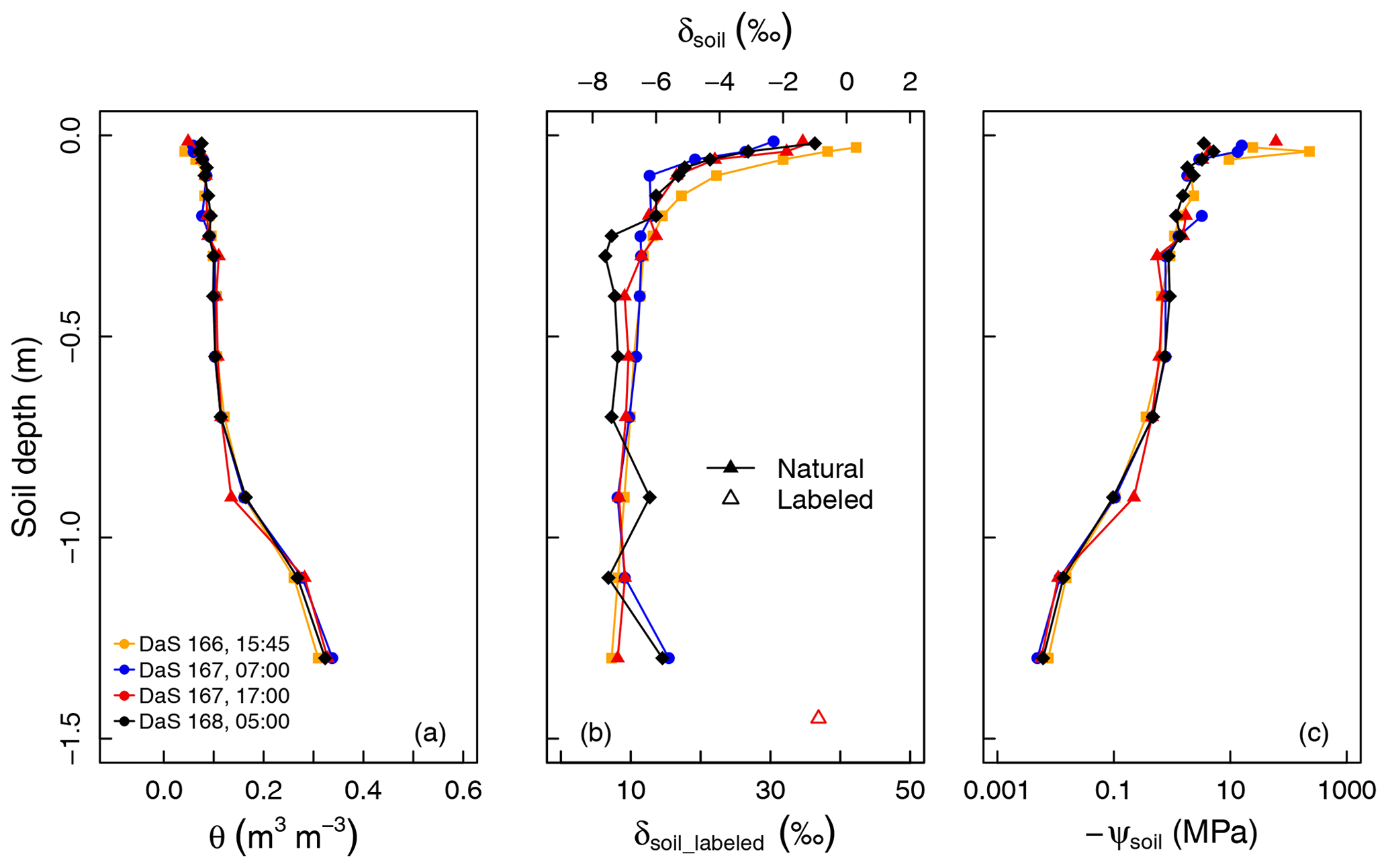
Figure 2(a) Measured soil volumetric water content (θ), (b) oxygen isotopic composition (δsoil), and (c) calculated soil matric potential (ψsoil) profiles during the sampling period.
Water in the top soil layers (−0.040 m < z < −0.015 m) was isotopically enriched (−3.2 ‰ < δsoil < 0.3 ‰) in contrast to the deepest layer ( ‰ ±0.30 ‰ at −1.30 m). Following the labeling of the reservoir water on DaS 166 at 17:00 LT, δsoil reached a value of 36.9 ‰ at −1.50 m on DaS 167 at 17:00 LT. The development of the vegetation on DaS 166–168 (LAI =5.6) and the observed surface θ values lead us to assume that the rhizotron water losses were solely due to transpiration flux (i.e., evapotranspiration equals transpiration). The soil water oxygen isotopic exponential-shaped profiles were due to fractionating evaporation flux and, to a great extent, the fact that the soil was bare or the tall fescue cover was not fully developed in the early stages of the experiment. Therefore, the differences in the soil water oxygen isotopic profile observed on the four different sampling dates were either due to lateral heterogeneity (e.g., upper soil layers), the soil capillary rise of labeled water from the reservoir (deep soil layers), or the hydraulic redistribution of water through roots (if the isotopic composition of the redistributed water differs from that of the soil water at the release location). We noted an isotopic enrichment of 1.0 ‰ of soil water observed on DaS 168 at 05:00 LT at a depth of −0.9 m with respect to the mean δsoil value across previous sampling dates. This could partly be due to factors such as the upward preferential flow of labeled water from the bottom soil layers and could, therefore, be a sign of the lateral heterogeneity of the soil. Another reason for this would be the hydraulic redistribution of labeled water by the roots. However, it was not possible to evaluate the relative importance of these three processes (lateral heterogeneity, capillary rise/preferential flow, and hydraulic redistribution) in the setting of the soil water isotopic profile, as the physically based soil–root model presented in section 2.4 does not account for soil liquid and vapor flow. This was also not the primary intent of the present study.
The observed RLD profile (Fig. 1a) showed a typical exponential shape, i.e., a maximum at the surface (5.42±0.34 cm cm−3) down to a minimum at −1.10 m (0.540±0.35 cm cm−3), and it increased again from the latter depth up to a value of 1.660 cm cm−3 at −1.30 m. This significant trend was most probably a direct consequence of the high soil water content value in this deeper layer.
3.1.2 Plant water and isotopic temporal dynamics
The temporal variation in δtiller (Fig. 3a) was found to be either (i) moderate during day and night, i.e., from DaS 167 at 06:00 to 11:00 LT ( ‰) and from DaS 167 at 21:30 LT to DaS 168 at 00:00 LT ( ‰), (ii) strong during the day, i.e., from DaS 167 at 11:00 to 18:00 LT (maximum value of 20.9 ‰ on DaS 167 at 12:40 LT), or (iii) strong during the night, i.e., from DaS 167 at 04:00 to 06:00 LT (maximum value of 36.4 ‰ on DaS 167 at 05:15 LT) and from DaS 168 at 00:00 to 06:00 LT (maximum value of 14.6 ‰ on DaS 168 at 04:00 LT). Note that transpiration (Fig. 3b) also occurred at night during the sampling period, due to the relatively high temperature in the glasshouse leading to a value of atmospheric relative humidity smaller than 85 % (Fig. 3b). From 12:00 to 14:00 LT and from 16:00 to 17:00 LT on DaS 167 (case ii), high values of leaf transpiration corresponded to high values of δtiller.
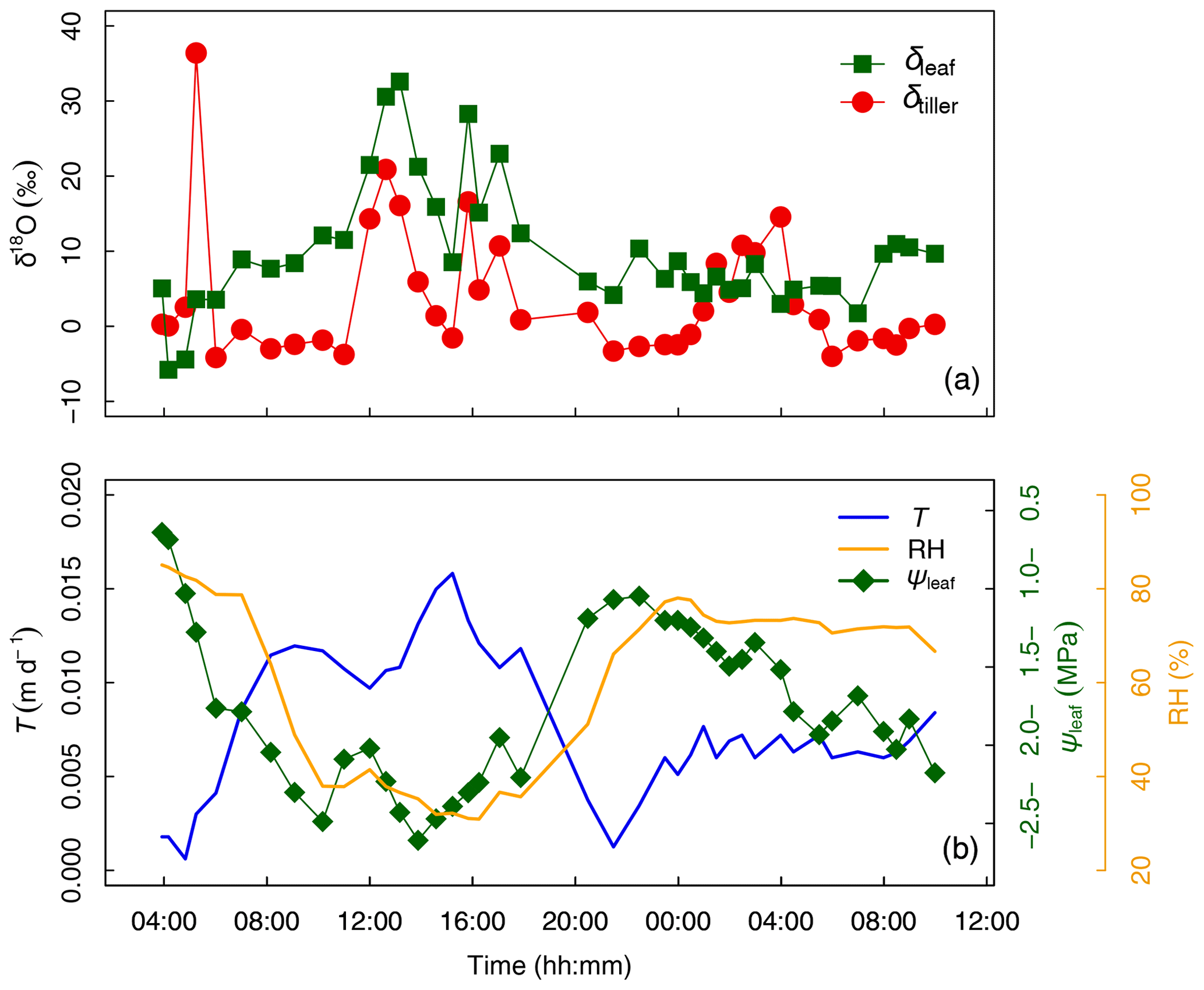
Figure 3(a) Time series of tiller and leaf water oxygen isotopic compositions (δtiller and δleaf, respectively, ‰). (b) Transpiration flux (T, in m d−1), relative humidity (HR, %), and leaf water potential (ψleaf, in MPa) from days after seeding (DaS) 167 at 04:00 LT to DaS 168 at 11:00 LT. Labeling was carried out on DaS 166 at 17:00 LT.
3.1.3 Partial decorrelation between water and isotopic state variables
Figure 4 shows that variables describing plant water status, i.e., T and RH (Fig. 4a) and T and ψleaf (Fig. 4b), were well correlated: the coefficient of determination (R2) was equal to 0.78 and 0.70 for the entire experimental duration, respectively. However, linear relationships between water status and isotopic variables were either nonexistent, e.g., between T and δtiller (R2=0.01, Fig. 4c) and between ψleaf and δtiller (R2=0.00, Fig. 4h), or characterized by a low R2 and high p value (e.g., between T and δleaf, R2=0.43, p > 0.05, Fig. 4d). The partial temporal disconnect between δleaf and T could not be attributed to problems with the isotopic methodology during processes such as the vacuum distillation of the water from the plant tillers and leaves: the water recovery rate was always greater than 99 % and Rayleigh distillation corrections (Dansgaard, 1964; Galewsky et al., 2016) were applied to standardize the observed oxygen isotopic composition values to a 100 % water recovery (based on the comparison of the sample weight loss during distillation and the mass of collected distilled water). The evolution of δleaf was strongly correlated with that of δtiller during the day (R2=0.90), whereas it was not correlated during the night (R2=0.00, Fig. 4j). These observed correlations are in agreement with the Craig and Gordon (1965) model revisited by Dongmann et al. (1974) and later by Farquhar and Cernusak (2005) and Farquhar et al. (2007). The model, which is extensively used in the current literature (e.g., Dubbert et al., 2017), states that, at isotopic steady-state, δleaf is a function of the input water oxygen isotopic composition (δtiller) among other variables, i.e., leaf temperature (not measured during the experiment), stomatal and boundary layer conductances, oxygen isotopic composition of atmospheric water vapor, and relative humidity.
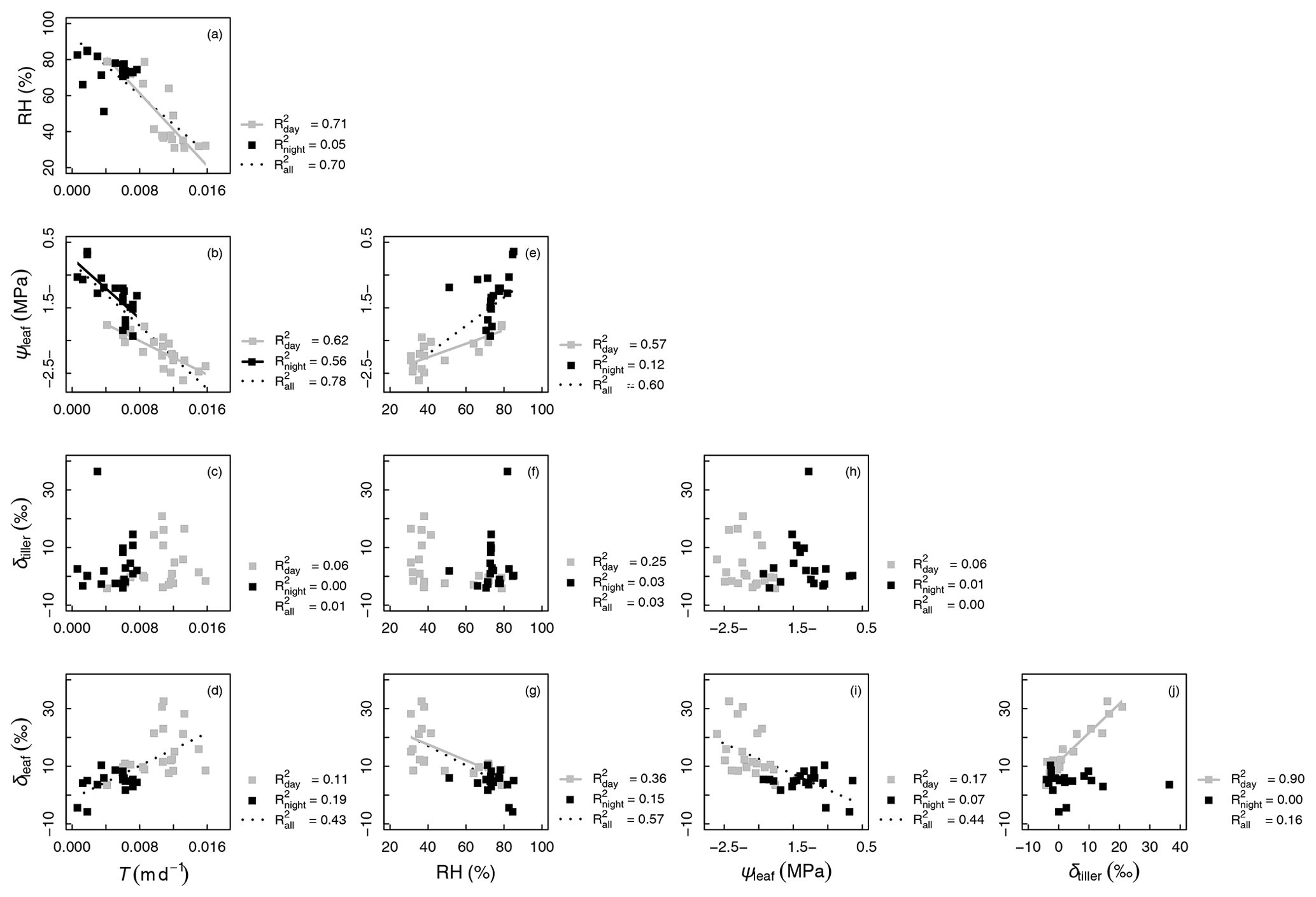
Figure 4Correlations between measured variables: oxygen isotopic compositions of xylem and leaf waters (δtiller and δleaf, respectively, in ‰), transpiration rate (T, in m d−1), relative humidity (RH, %), and leaf water potential (ψleaf, in MPa). The coefficients of determination (R2 values) are reported for all data as well as separately for “day” (gray symbols) and “night” data (black symbols; see Appendix C for definition of “day” and “night” experimental periods). Regression lines are drawn for linear models with a p value < 0.01
It is generally difficult to observe a statistically significant δleaf−δtiller (Fig. 4j) relationship at this temporal scale under natural abundance conditions in the field, as the soil water isotopic weak gradient translates into weaker δtiller temporal dynamics. The quality of the linear fit between δleaf and δtiller data collected during the day (R2=0.90) was made possible in this specific experiment by the artificial isotopic labeling pulse that enhanced the soil water isotopic gradient, which in turn increased the range of variation in δtiller, ultimately highlighting the δleaf−δtiller temporal correlation. Air relative humidity is a driving variable of δleaf in the model of Dongmann et al. (1974) via the competing terms of (1− RH) ⋅δtiller and RH ⋅δatm, where δatm is the atmospheric water vapor isotopic composition inside the glasshouse. An overall significant linear correlation was observed between RH and δleaf during the experiment (R2=0.57, Fig. 4g). During the two night periods (i.e., from 04:00 to 06:00 LT and from 20:30 to 07:00 LT), as relative humidity increased in the glasshouse (51 % < RH < 85 %, Fig. 3b), the influence of the isotopic labeling of the tiller water (due to the labeling of deep soil water) via the (1− RH) ⋅δtiller term decreased to the benefit of the RH ⋅δatm term (with δatm values ranging from −15.9 to −10.7 ‰ and a mean of ‰, data not shown). This was especially visible between 04:50 and 06:00 LT on DaS 167 and between 01:00 and 06:00 LT on DaS 168, when δtiller reached greater values than δleaf.
From a different perspective, as three plant water samples were pooled to reach a workable volume for the isotopic analysis at each observation time without replicates, the isotopic signal fluctuations may reflect both its temporal dynamics and its variability within the plant population.
3.2 Simulations
This section focuses on modeling results with (i) an explanation of the variability of plant and soil observations, (ii) an independent validation of model predictions, (iii) a discussion of possible sources of variability not accounted for by the model, and (iv) a comparison of physical and Bayesian model outputs.
3.2.1 Rooting depth and transpiration rate control δtiller and ψleaf fluctuations, respectively
Despite the use of a global optimizer and 4 degrees of freedom (Lpr, kaxial, ksat, and λ, see optimal values in Table 1) that specifically aimed at matching the simulated and observed temporal dynamics of δtiller, none of the 60 root system groups or the average population could reproduce the measured fluctuations in time (R2=0.00, Fig. 5a), regardless of the weight attributed to this criterion in the objective function. The predicted versus the observed δtiller distributions including all plant groups and observation times differed noticeably but not significantly (6.6±8.4 ‰ and 3.7±8.4 ‰, respectively) when pooling three simulated δtiller randomly at each observation time (P > 0.01 in 92 cases out of 100 repeated drawings), as in the measurements. In addition, the simulated ψleaf fitted the observations well (R2=0.67, with overall distributions of MPa and MPa, respectively; Fig. 5c). When analyzing the distributions of ψleaf and δtiller per maximum root system depth (Fig. 5b, d), it appears that the ψleaf signal is not sensitive to the rooting depth (Fig. 5d), whereas δtiller is more sensitive to rooting depth than to the temporal evolution of the plant environment (Fig. 5b).
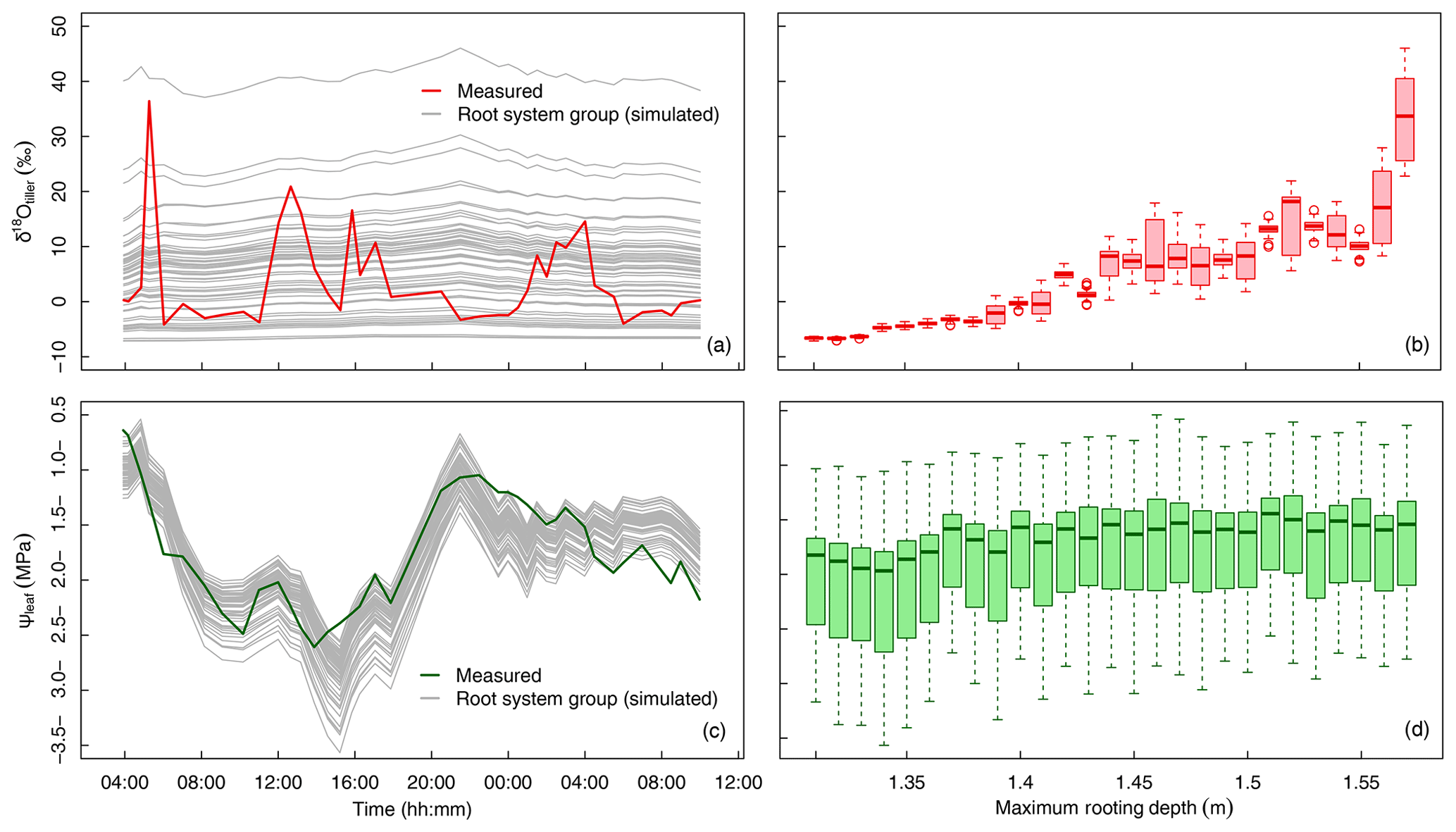
Figure 5Variation in δtiller and ψleaf in time and across the 60 groups of simulated root systems. (a) The measured (thick red line) and simulated (thin gray lines, one line per root system group, following a “swarm” pattern) temporal dynamics of δtiller. (b) Boxplot of simulated δtiller values for each root system maximum depth, in 1 cm increments. (c) The measured (thick green line) and simulated (thin gray lines, one line per root system group, following a “roller-coaster” pattern) temporal dynamics of ψleaf. (d) Boxplot of simulated ψleaf values for each root system maximum depth, in 1 cm increments.
Table 1Optimum and limits of the four-dimensional parametric space explored by the global optimization algorithm aiming at minimizing the difference between simulated and observed δtiller and ψleaf, as well as their standard deviation from average values during the full experiment.
This leaves us with two hypotheses. First, the “roller-coaster hypothesis” states that δtiller rapidly goes up and down with all individuals onboard the same car (i.e., little variability within the population, unlike the predictions in Fig. 5a but similar to the simulated ψleaf in Fig. 5c). If this holds true, the physical model lacks a process that would capture the observed temporal fluctuations of δtiller. Second, the “swarm pattern hypothesis” states that δtiller is rather stable in time, but its values within the plant population are dispersed like a flying swarm; thus, δtiller values sampled at different times fluctuate, not due to temporal dynamics but instead owing to the fact that different individuals are sampled (Fig. 5a).
The model suggests that the tall fescue population ψleaf follows a “roller-coaster” dynamics that is driven by transpiration rate, whereas the population δtiller follows a “swarm” pattern that is driven by the maximum rooting depth of the sampled plants. As no correlation could be expected between the drivers (the maximum rooting depth of the sample plants and the canopy transpiration rate), our analysis explains the absence of a correlation between δtiller and ψleaf or transpiration rate.
In future experiments and in the specific context of labeling pulses, sampling more plants at each observation time would help disentangle the spatial from the temporal sources of variability of ψleaf and δtiller. However, it would be at the cost of the temporal resolution of observations or would necessitate a larger setup with more plants in the case of controlled conditions experiments.
3.2.2 Independent observations support the validity of the hydraulic model predictions
In the last 12 h of the experiment (DaS 167 at 17:00 LT to DaS 168 at 05:00 LT), the measured soil water content increased by 0.029 m3 m−3 at a depth of −0.9 m, which could be a sign of nighttime hydraulic redistribution. During the same period, the physical model predicted a cumulative water exudation sufficient to increase soil water content by 0.003 m3 m−3, as the soil water potential was low enough to generate reverse flow but high enough not to disrupt the hydraulic continuity between the soil and roots (Carminati and Vetterlein, 2013; Meunier et al., 2017a). While this increase is smaller than the observed water content change, it is only a component in the soil water mass balance. Given the soil water potential vertical gradient, upward soil capillary water flow may have accounted for another part of the observed moisture change. Experimental observations also show that δsoil increased by 1.0 ‰ at a depth of −0.9 m during that time (−6.2 ‰, which was a value significantly higher than −7.1 ‰ ±0.1 ‰ at earlier times based on an ANOVA analysis, P < 0.01), whereas our simulations of hydraulic redistribution generated a 0.34 ‰ increase of δsoil. As soil capillary flow may not generate local maxima of δsoil (no enrichment observed at surrounding depths, see Fig. 2b), and soil evaporation is assumed negligible at that depth, it is likely that the observed local enrichment was entirely due to hydraulic redistribution, which would then be underestimated by a factor of about 3 in our simulations. Increasing water exudation by a factor 3 would imply a simulated water content change due to exudation of 0.0090 m3 m−3 absolute water content, which remains compatible with the experimental observation. Between a depth of −1.1 m and −0.9, the nighttime water flow pattern transitioned from exudation to uptake in both measurements and predictions. At −1.1 m, the model predicted a cumulative water uptake sufficient to decrease the soil water content by 0.0101 m3 m−3, compared with the observed 0.0141 m3 m−3 total soil water content decrease. The remaining 0.004 m3 m−3 water content decrease may have contributed to the recharge of the soil layers above via capillary flow, which was not simulated. Therefore, all relevant measurements (local increase in soil water content and local enrichment of water isotopic composition) and simulation results (S < 0, i.e., local water release from roots) clearly converge to the conclusion that hydraulic lift occurred in the vicinity of a depth of −0.9 m in the early morning of DaS 168.
As far as fitted parameter values are concerned, Lpr ( m MPa−1 s−1) was in the range found by Martre et al. (2001) for tall fescue ( m MPa−1 s−1) and also falls in the range obtained by Meunier et al. (2017a) for another grass (Lolium multiflorum Lam., to m MPa−1 s−1). Our kaxial value cannot be compared to values of axial root conductance from the literature, as it transfers the water absorbed by roots in a single “big root” per group of five identical plants. The optimal value of ksat was quite high (Table 1) but reportedly very correlated with λ (i.e., soil unsaturated hydraulic conductivity is proportional to ksat but also to ; van Genuchten, 1980), so that the low value of the latter compensated for the high value of the former; thus, they should be considered as effective rather than physical parameters.
3.2.3 Other sources of variability and observational error
Our treatment of the soil medium in this experiment (sieving and irrigation from the bottom) makes it laterally more homogeneous than natural soils. This method allowed us to specifically study the impact of the vertical gradients of δsoil on δtiller. It also justified the use of a simplistic one-dimensional model adapted to the vertically resolved measurements. If lateral heterogeneity of soil water content remained and was accounted for, our predictions of root water uptake distribution, δtiller, and ψleaf would be altered. Observational errors in the gravimetric soil water content measurement (converted to soil water potential using the soil water retention curve) would also alter these predictions. In order to quantify the sensitivity of our simulated results to such heterogeneity or observational error, we varied the soil water content input by ±0.02 m3 m−3 at three critical depths (−0.9, −1.1, and −1.3 m, before interpolation) at the last observation time, during which measurements and simulations suggested that hydraulic lift occurred. Our results were mostly sensitive to soil water content alterations at −0.9 m, and they barely differed in response to alterations at −1.1 and −1.3 m, although the conclusions were not affected qualitatively. No statistically significant difference between the predicted and observed δtiller distributions for the overall dataset could be found when pooling three simulated δtiller randomly at each observation time (predicted and observed δtiller distributions were closest to differing when the soil water content was reduced by 0.02 m3 m−3 at a depth of 0.9 m; P > 0.01 in 76 cases out of 100 repeated drawings). Measured and simulated ψleaf remained very correlated in all cases (from an R2 value of 0.69 to 0.74 when adding or removing 0.02 m3 m−3 at a depth of 0.9 m, respectively). Furthermore, when adding or removing 0.02 m3 m−3 at a depth of 0.9 m, cumulative water exudation at −0.9 m varied between 0.0019 and 0.0035 m3 m−3, uptake at −1.1 m varied between 0.0080 and 0.0108 m3 m−3, and the simulated change in the δsoil ranged between 0.28 and 0.40 ‰, respectively.
Lateral heterogeneity in the soil water isotopic composition may as well occur at the microscopic scale. As water in micropores is less mobile than water in meso- and macropores (Alletto et al., 2006), it is likely that, in the lower half of the profile, the capillary rise of labeled water affected the composition of water in meso- and macropores more than in micropores. If roots have more access to meso- and macropore water, then the water absorbed by roots would be isotopically enriched compared with the “bulk soil water” characterized experimentally. The importance of this possible bias depends on soil texture and heterogeneity (e.g., the existence of more isolated “pockets” of soil or compact clusters) as well as on the speed of water mixing between mobile and immobile water fractions (Gazis and Feng, 2004). Including this process in the modeling would necessitate sufficient observations to estimate the aforementioned properties and ideally some quantification of the lateral heterogeneity of the soil water isotopic composition at the microscale.
The lateral heterogeneity of soil hydraulic properties and root distribution may also have participated in the generation of lateral soil water potential heterogeneities, particularly in undisturbed soils. If one had access to data on the lateral heterogeneity of soil properties and rooting density, it would be possible to simulate three-dimensional soil–root water flow with a tool such as R-SWMS (modeling “Root-Soil Water Movement and Solute transport”; Javaux et al., 2008), using a randomization technique for soil properties' distribution as in Kuhlmann et al. (2012), in order to obtain estimations of the relative importance of this type of heterogeneity on δtiller and ψleaf variability.
Unlike the tiller water isotopic composition, the leaf water potential turned out to be very sensitive to the transpiration rate in our simulations (see temporal fluctuations of gray lines in Fig. 5c) and not very sensitive to the root distribution (see small variations in leaf water potential across individuals in Fig. 5d). In this setup, this suggests that the hydraulic conductance of the soil–root system limited the shoot water supply more than the distribution of roots, as in Sulis et al. (2019). Simulated baseline (i.e., for uniform transpiration rates) leaf water potentials are shown as gray lines in Fig. 5c, and measured leaf water potentials are shown as a green line in the same panel. The fact that they match well, despite the high sensitivity of the leaf water potential to the transpiration rate, reinforces the idea that the transpiration rate was likely not spatially heterogeneous among the plant population. Therefore, the tiller water isotopic composition, whose sensitivity to the transpiration rate is already very low, was likely not affected by transpiration rate heterogeneity.
3.2.4 Do root water uptake profiles predicted by hydraulic and Bayesian models differ?
The root water uptake dynamics predicted by the mechanistic model are shown in Fig. 6a. The overall pattern of peaking water uptake in the lower part of the profile during daytime matched that of the statistical model, and the correlation coefficient of both model predictions was relatively high (R2=0.53) on average over the simulation period (see Fig. 7). The main differences were as follows: (i) in the upper soil layers where the soil water potential was lower than −1.5 MPa, the statistical model predicted water uptake, which is theoretically impossible given the leaf water potential above −0.4 MPa (van Den Honert, 1948); (ii) in the upper half of the profile, the physical model predicted exudation at a rate limited by the low hydraulic conductivity between the root surface and the bulk soil, with a peak at night, at a depth of −0.9 m (quantitative analysis in previous section); (iii) below a depth of −1.0 m, the water uptake rate predicted by the statistical model steadily increased with depth while that of the physical model was more uniform, likely due to axial hydraulic limitation (e.g., Bouda et al., 2018) counteracting the increasing soil water potential with depth. Note that the outcome of the statistical model may significantly depend on the definition of the a priori relative RWU (rRWU) profile. In the present study, we set it to follow a “flat” uniform distribution (i.e., rRWUj ; see Appendix E); in other words, each layer was initially defined to contribute equally to RWU. Contrary to other studies (e.g., Mahindawansha et al., 2018), where the a priori rRWU profile was empirically constructed on the basis of soil water content and root length density profiles, we decided not to further arbitrarily constrain the Bayesian model for the sake of comparison with the physically based soil–root model.

Figure 6Time series of the profiles of root water uptake per unit soil volume (sink term, d−1) computed with the physically based model. (a) Sum of sink terms across the 60 groups of the population. (b) Variability of the sink terms within the 60 groups of the population (1 standard deviation).
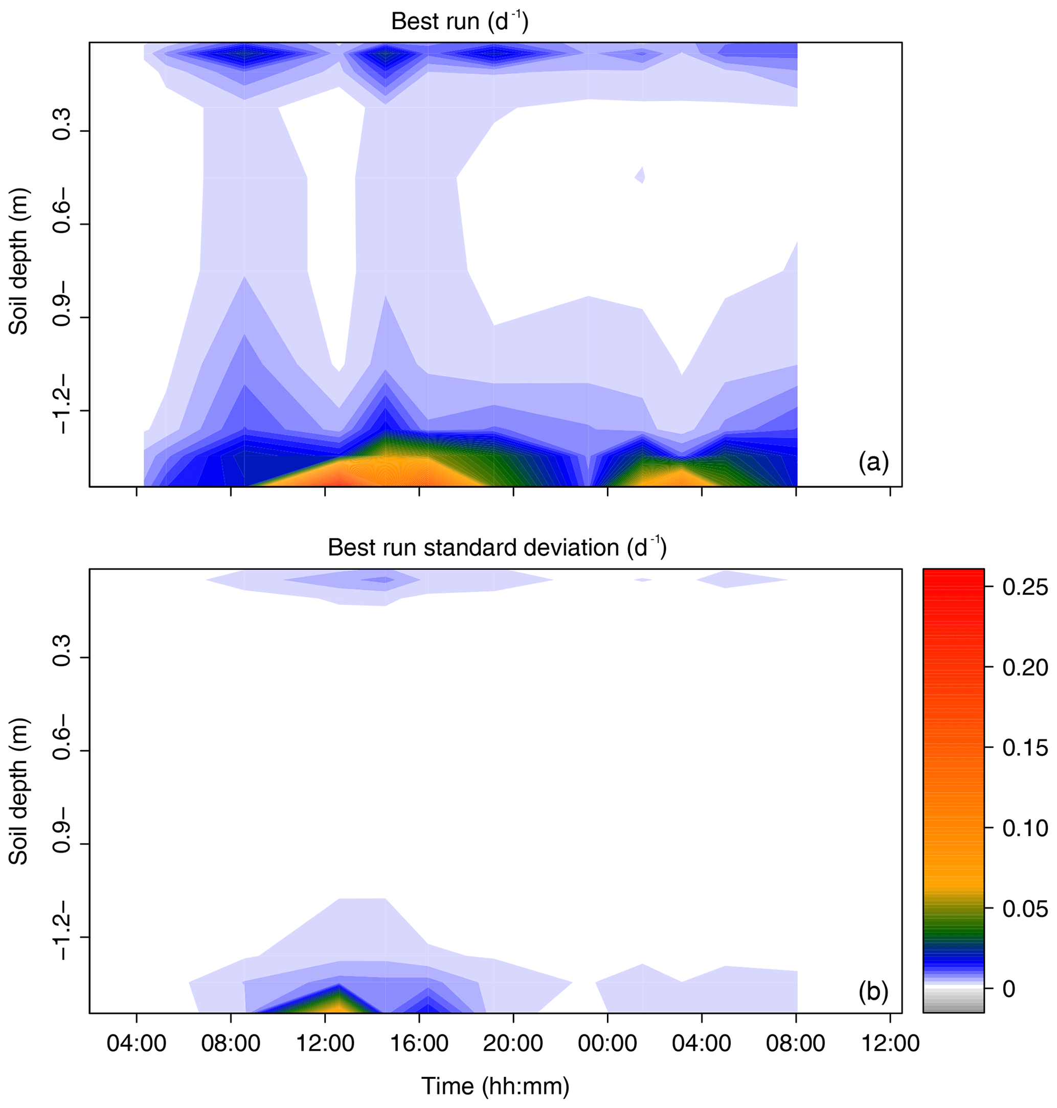
Figure 7Time series of the profiles of root water uptake per unit soil volume (sink term, d−1) computed with the statistical model SIAR (a). Panel (b) reports the variance of the estimated sink term (1 standard deviation).
3.3 Progress and challenges in soil water isotopic labeling for RWU determination
Often, in the field, the vertical dynamics of both soil water oxygen and hydrogen isotopic compositions are not strong enough (or show convolutions leading to issues of identifiability) for partitioning RWU among different contributing soil water sources. As a consequence, we unfortunately cannot make use of the natural variability in isotopic abundances for deciphering soil–root transfer processes (Beyer et al., 2018; Burgess et al., 2000). To address this limitation of the isotopic methodology, labeling pulses have been applied locally at different depths in the soil profile (e.g., Beyer et al., 2016) or at the soil upper/lower boundaries under both laboratory and field conditions by mimicking rain events Piayda (e.g., Piayda et al., 2017) and/or rise of the groundwater table (Meunier et al., 2017a; Kühnhammer et al., 2019).
After labeling, we are faced with two problems. First, the labeling pulse might enhance RWU at the labeling location if the volume of added water significantly changes the value of soil water content. This, therefore, poses the question of the meaningfulness of the derived RWU profiles, irrespective of the model used (i.e., physically based soil–root model or statistical multisource mixing model). In other words, are we observing natural RWU behavior of the plant individual or population or are we seeing the influence of the labeling pulse? Thus, a way to move forward is the utilization of environmental observatories such as ecotrons and field lysimeters (e.g., Groh et al., 2018; Benettin et al., 2018) that provide the means to better constrain hydraulic boundary conditions and reduced their isotopic heterogeneity. They allow for a mechanistic and holistic understanding of soil–root processes from stable isotopic analysis.
Second, the difficulty to properly observe the propagation of the labeling pulse in the soil after application and the temporal dynamics of the plant RWU isotopic composition in situ is also problematic. Beyer and Dubbert (2019) presented a comprehensive review on recent isotopic techniques for nondestructive, online, and continuous determination of soil and plant water isotopic compositions (e.g., Rothfuss et al., 2013; Quade et al., 2019; Volkmann et al., 2016a) as alternatives to the widely used combination of destructive sampling and offline isotopic analysis following cryogenic vacuum extraction (Orlowski et al., 2016) or liquid–vapor direct equilibration (Wassenaar et al., 2008). These techniques have the potential for a paradigm change in isotopic studies on RWU processes so that, for example, isotopic effects during sample collection are fully understood.
The present study highlights that the isotope data alone should not be “trusted” and should always be complemented by information on environmental factors as well as soil and plant water status in order to go beyond the simple application of statistical models. This is especially the case in the framework of labeling studies where strong soil water isotopic gradients may induce strong dynamics of the RWU isotopic composition from a low variability of rooting depths.
In the present study, light could be shed on RWU of Festuca arundinacea by specifically manipulating the lower boundary conditions for water content and oxygen isotopic composition. The new version of the one-dimensional model of Couvreur et al. (2014) implemented here accounted for both root and soil hydraulics in a population of “big” root systems of known root length density profile. This approach underlined the high sensitivity of δtiller to rooting depth and suggested that if δtiller is measured on a limited number of individuals, its variations in time may reflect the heterogeneity of the rooting depth within the population rather than temporal dynamics, which was minor in our simulations. The model avoided the prediction of water uptake at locations where it was physically unavailable (e.g., in the top half of the soil profile), by accounting for water potential differences observed between the leaves and the soil, and quantitatively explained the local isotopic enrichment of soil water as the occurrence of nighttime hydraulic lift at a depth of −0.9 m. Conversely, the Bayesian statistical approach tested for comparison, which was driven solely by isotopic information, naturally translated the observed changes of δtiller into profound temporal dynamics of RWU at the expense of ecophysiological considerations (e.g., the temporal dynamics of leaf water potential and transpiration rate).
This case study highlights the potential limitations of water isotopic labeling techniques for studying RWU: the soil water isotopic artificial gradients induced from water addition result in an improvement in RWU profiles' determination such that they are properly characterized spatially and temporally. As already pointed out in the review of Rothfuss and Javaux (2017), this study also underlines the interest of complementing in situ isotopic observations in soil and plant water with information on soil water status and plant ecophysiology. Furthermore, this work calls for the use of simple soil–root models (although they require additional water status measurements and make more explicit assumptions on the description of the soil–plant system than the traditional Bayesian approach) for inversing isotopic data and gaining insights into the RWU process.
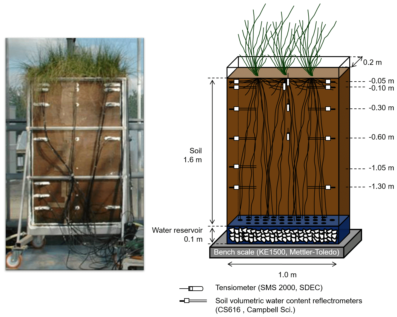
Table B1Soil retention curve and parameters' optimized values (van Genuchten, 1980 – Burdine; Meunier et al., 2017a).
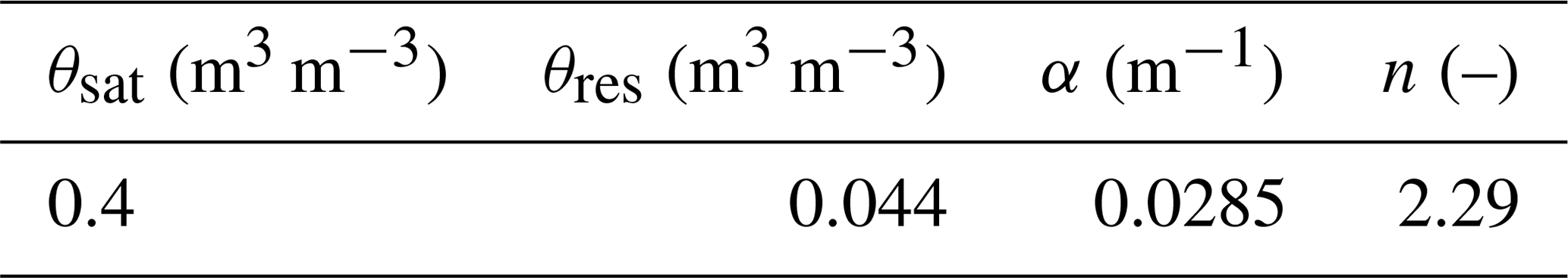
Table C1Timeline of the destructive sampling. DaS stands for “day after seeding”. The “day” periods are from 07:00 to 17:50 LT on DaS 167 and from 07:00 to 10:00 LT on DaS 168. The “night” periods are from 03:55 to 06:00 LT on DaS 167 and from 20:30 to 06:00 LT on DaS 167–168.
The parametrization method used in this study was inverse modeling, and there were four targets: (i) minimizing the differences between observed and predicted δtiller in each pool (p), (ii) minimizing the difference between the standard deviations of observed and predicted δtiller (temporal and population deviations combined), (iii) minimizing the differences between observed and predicted ψleaf in each root system group (i), and (iv) minimizing the difference between the standard deviations of observed and predicted δtiller (temporal and population deviations combined). These targets were translated into an objective function (OF) to be minimized, where the differences were normalized by the standard deviation (SD) of the observations in order to make the error function dimensionless:
where Np is the number of δtiller pools simulated (100) at each observation time, Ni is the number of plant groups simulated (60), and Nt is the total number of observation times (40).
The global optimizer multistart heuristic algorithm OQNLP (Optimal Methods Inc.) from the MATLAB (MathWorks, Inc., USA) optimization toolbox was used to minimize the error function within the lower and upper limits of the parametric space reported in Table 1.
The Bayesian inference statistical model SIAR (Parnell et al., 2013) was used to determine the profiles of relative contributions of 10 identified potential water sources to RWU (rRWU, dimensionless). These water sources were defined as originating from the following soil layers: 0.00–0.03, 0.03–0.07, 0.07–0.15, 0.15–0.30, 0.30–0.60, 0.60–0.90, 0.90–1.20, 1.20–1.32, 1.32–1.37, and 1.37–1.44 m. Their corresponding isotopic compositions were obtained from the measured soil water isotopic compositions (δsoil) and volumetric content (θ) values following Eq. (E1) (Rothfuss and Javaux, 2017):
where J is the soil layer index, j is the soil sub-layer index, and ΔZj is the thickness of the soil sub-layer j. Therefore, Eq. (E1) translates the soil water isotopic composition measured across sub-layers j into representative isotopic compositions of the different sources (i.e., across layers J). The computed δsoil,J values were compared to δtiller values. For this comparison, δtiller measurements were pooled into 12 groups corresponding to different time periods. These groups were defined to best reflect the apparent temporal dynamics of δtiller.
For each of the 12 time periods the following actions were undertaken:
- i.
the “siarmcmcdirichletv4” function of the SIAR R package (https://cran.r-project.org/web/packages/siar/index.html, last access: 15 August 2019) was run 500 000 times with prescribed burnin and thinby equal to 50 000 and 15, respectively, and the output of the model (i.e., the a posteriori rRWU distribution across the 10 soil water sources, J) was obtained from a flat Dirichlet a priori rRWU distribution (i.e., rRWU);
[ii.] the “best run” (br, dimensionless) was selected from SIAR's output. It was defined as the closest solution of the relative contributions across sources from the set of most frequent values (mfv, dimensionless), i.e., the relative contribution with the greatest probability of occurrence. The best run was identified as minimizing the objective function shown below, i.e., the RMSE (root mean square error) with respect to the set of mfvJ:
- iii.
br was then multiplied by the transpiration rate (in m d−1) and divided by the soil layer thicknesses (ΔZJ, in m) to obtain the sink terms (SJ, i.e., root water uptake rate per unit soil volume, expressed in d−1). The interest of sink terms in a comparison is that they do not vary with soil vertical discretization.
Steps (i)–(iii) were repeated 1000 times to estimate the variance in the best run for each time period and soil water source J.
| Name | Symbol | Units |
| Leaf water potential/head | ψleaf | (MPa) |
| Soil water potential/head | ψsoil | (MPa) |
| Water volumetric mass | ρw | (kg m−3) |
| Soil apparent density | ρb | (kg m−3) |
| Soil gravimetric water content | θgrav | (kg kg−1) |
| Soil volumetric water content | θ | (m3 m−3) |
| Intensity of water uptake (sink term) | S | (d−1) |
| Transpiration rate per unit soil area | T | (m d−1) |
| Air relative humidity | RH | % |
| Soil horizontal area | Asoil | (m2) |
| Soil layer depth (for each layer) | z | (m) |
| Soil layer thickness (for each layer) | ΔZ | (m) |
| Root length (for each soil layer) | lroot | (m) |
| Relative root water uptake | rRWU | (Dimensionless) |
| Best run | br | (Dimensionless) |
| Root length density | RLD | (m m−3) |
| Soil water oxygen isotopic composition | δsoil | (‰) |
| Tiller water oxygen isotopic composition | δtiller | (‰) |
| Leaf water oxygen isotopic composition | δleaf | (‰) |
| Soil–root system conductance | Ksoil–root | (m3 MPa−1 s−1) |
| Soil–root radial conductance | Kradial | (m3 MPa−1 s−1) |
| Root radial conductivity | Lpr | (m MPa−1 s−1) |
| Root axial conductance | Kaxial | (m3 MPa−1 s−1) |
| Equivalent root axial conductivity | kaxial | (m4 MPa−1 s−1) |
| Soil hydraulic conductivity | ksoil | (m2 MPa−1 s−1) |
| Saturated soil hydraulic conductivity | ksat | (m2 MPa−1 s−1) |
| Soil hydraulic conductivity parameter | λ | (Dimensionless) |
| Soil relative water content | Se,j | (Dimensionless) |
Upon acceptance, all of the research data that were required to create the plots will be available from reliable FAIR-aligned data repositories with assigned DOIs.
TB, JLD, and PB designed the experiments, and TB, JLD, PB, and YR carried them out. VC, FM, and MJ developed the physically based root water uptake model code, and VC and FM performed the simulations. YR performed the statistical simulations. VC, YR, FM, and MJ prepared the paper with contributions from all co-authors.
The authors declare that they have no conflict of interest.
This experiment was part of the “Charactérisation biogéochimique de l'ASCenceur HYDraulique” (ASCHYD) project and was supported by the French Institut national des sciences de l'Univers (INSU) in the framework of the thematic action BIOgéochimie, HydrologiE et Fonctionnement des ECosysTèmes (BIOHEFECT) of the Ecosphère Continentale et Côtière (EC2CO) initiative. Valentin Couvreur was supported by the Belgian National Fund for Scientific Research (FNRS; grant no. FC 84104), the Interuniversity Attraction Poles Program of the Belgian Science Policy Office (grant no. IAP7/29) and the Communauté française de Belgique-Actions de Recherches Concertées (grant no. ARC16/21-075). Félicien Meunier was first funded by the Belgian American Educational Foundation (BAEF) and the Wallonie-Bruxelles International (WBI) and subsequently by the Research Foundation – Flanders (FWO) as a junior postdoc.
This paper was edited by Markus Weiler and reviewed by Matthias Beyer and two anonymous referees.
Alletto, L., Coquet, Y., Vachier, P., and Labat, C.: Hydraulic conductivity, immobile water content, and exchange coefficient in three soil profiles, Soil Sci. Soc. Am. J., 70, 1272–1280, https://doi.org/10.2136/sssaj2005.0291, 2006.
Benettin, P., Volkmann, T. H. M., von Freyberg, J., Frentress, J., Penna, D., Dawson, T. E., and Kirchner, J. W.: Effects of climatic seasonality on the isotopic composition of evaporating soil waters, Hydrol. Earth Syst. Sci., 22, 2881–2890, https://doi.org/10.5194/hess-22-2881-2018, 2018.
Beyer, M. and Dubbert, M.: X Water Worlds and how to investigate them: A review and future perspective on in situ measurements of water stable isotopes in soils and plants, Hydrol. Earth Syst. Sci. Discuss., https://doi.org/10.5194/hess-2019-600, in review, 2019.
Beyer, M., Koeniger, P., Gaj, M., Hamutoko, J. T., Wanke, H., and Himmelsbach, T.: A deuterium-based labeling technique for the investigation of rooting depths, water uptake dynamics and unsaturated zone water transport in semiarid environments, J. Hydrol., 533, 627–643, https://doi.org/10.1016/j.jhydrol.2015.12.037, 2016.
Beyer, M., Hamutoko, J. T., Wanke, H., Gaj, M., and Koeniger, P.: Examination of deep root water uptake using anomalies of soil water stable isotopes, depth-controlled isotopic labeling and mixing models, J. Hydrol., 566, 122–136, https://doi.org/10.1016/j.jhydrol.2018.08.060, 2018.
Bouda, M., Brodersen, C., and Saiers, J.: Whole root system water conductance responds to both axial and radial traits and network topology over natural range of trait variation, J. Theor. Biol., 456, 49–61, https://doi.org/10.1016/j.jtbi.2018.07.033, 2018.
Burgess, S. S. O., Adams, M. A., Turner, N. C., and Ward, B.: Characterisation of hydrogen isotope profiles in an agroforestry system: implications for tracing water sources of trees, Agr. Water Manage., 45, 229–241, https://doi.org/10.1016/S0378-3774(00)00105-0, 2000.
Carminati, A. and Vetterlein, D.: Plasticity of rhizosphere hydraulic properties as a key for efficient utilization of scarce resources, Ann. Bot., 112, 277–290, https://doi.org/10.1093/aob/mcs262, 2013.
Couvreur, V., Vanderborght, J., and Javaux, M.: A simple three-dimensional macroscopic root water uptake model based on the hydraulic architecture approach, Hydrol. Earth Syst. Sci., 16, 2957–2971, https://doi.org/10.5194/hess-16-2957-2012, 2012.
Couvreur, V., Vanderborght, J., Beff, L., and Javaux, M.: Horizontal soil water potential heterogeneity: simplifying approaches for crop water dynamics models, Hydrol. Earth Syst. Sci., 18, 1723–1743, https://doi.org/10.5194/hess-18-1723-2014, 2014.
Craig, H. and Gordon, L. I.: Deuterium and oxygen-18 variations in the ocean and the marine atmosphere, Paper presented at the Stable Isotopes in Oceanographic Studies and Paleotemperatures, Spoleto, Italy, 1965.
Dansgaard, W.: Stable Isotopes in Precipitation, Tellus, 16, 436–468, https://doi.org/10.1111/j.2153-3490.1964.tb00181.x, 1964.
Dongmann, G., Nurnberg, H. W., Forstel, H., and Wagener, K.: On the Enrichment of in Leaves of Transpiring Plants, Radiat. Environ. Biophy., 11, 41–52, https://doi.org/10.1007/Bf01323099, 1974.
Dubbert, M. and Werner, C.: Water fluxes mediated by vegetation: emerging isotopic insights at the soil and atmosphere interfaces, New Phytol., 221, 1754–1763, https://doi.org/10.1111/nph.15547, 2019.
Dubbert, M., Kübert, A., and Werner, C.: Impact of Leaf Traits on Temporal Dynamics of Transpired Oxygen Isotope Signatures and Its Impact on Atmospheric Vapor, Font. Plant Sci., 8, 5, https://doi.org/10.3389/fpls.2017.00005, 2017.
Durand, J. L., Bariac, T., Ghesquiere, M., Biron, P., Richard, P., Humphreys, M., and Zwierzykovski, Z.: Ranking of the depth of water extraction by individual grass plants, using natural 18O isotope abundance, Environ. Exp. Bot., 60, 137–144, https://doi.org/10.1016/j.envexpbot.2006.09.004, 2007.
Fan, J. L., McConkey, B., Wang, H., and Janzen, H.: Root distribution by depth for temperate agricultural crops, Field Crops Res., 189, 68–74, https://doi.org/10.1016/j.fcr.2016.02.013, 2016.
Farquhar, G. D. and Cernusak, L. A.: On the isotopic composition of leaf water in the non-steady state, Funct. Plant Biol., 32, 293–303, https://doi.org/10.1071/Fp04232, 2005.
Farquhar, G. D., Cernusak, L. A., and Barnes, B.: Heavy water fractionation during transpiration, Plant Physiol., 143, 11–18, 2007.
Galewsky, J., Steen-Larsen, H. C., Field, R. D., Worden, J., Risi, C., and Schneider, M.: Stable isotopes in atmospheric water vapor and applications to the hydrologic cycle, Rev. Geophys., 54, 809–865, https://doi.org/10.1002/2015rg000512, 2016.
Gazis, C. and Feng, X. H.: A stable isotope study of soil water: evidence for mixing and preferential flow paths, Geoderma, 119, 97–111, https://doi.org/10.1016/S0016-7061(03)00243-X, 2004.
Gonfiantini, R.: Standards for stable isotope measurements in natural compounds, Nature, 271, 534–536, https://doi.org/10.1038/271534a0, 1978.
Gonzalez-Dugo, V., Durand, J. L., Gastal, F., and Picon-Cochard, C.: Short-term response of the nitrogen nutrition status of tall fescue and Italian ryegrass swards under water deficit, Aust. J. Agr. Res., 56, 1269–1276, https://doi.org/10.1071/Ar05064, 2005.
Groh, J., Stumpp, C., Lucke, A., Putz, T., Vanderborght, J., and Vereecken, H.: Inverse Estimation of Soil Hydraulic and Transport Parameters of Layered Soils from Water Stable Isotope and Lysimeter Data, Vadose Zone J., 17, https://doi.org/10.2136/vzj2017.09.0168, 2018.
Grossiord, C., Gessler, A., Granier, A., Berger, S., Brechet, C., Hentschel, R., Hommel, R., Scherer-Lorenzen, M., and Bonal, D.: Impact of interspecific interactions on the soil water uptake depth in a young temperate mixed species plantation, J. Hydrol., 519, 3511–3519, https://doi.org/10.1016/j.jhydrol.2014.11.011, 2014.
Javaux, M., Schroder, T., Vanderborght, J., and Vereecken, H.: Use of a three-dimensional detailed modeling approach for predicting root water uptake, Vadose Zone J., 7, 1079–1088, https://doi.org/10.2136/Vzj2007.0115, 2008.
Jesch, A., Barry, K. E., Ravenek, J. M., Bachmann, D., Strecker, T., Weigelt, A., Buchmann, N., de Kroon, H., Gessler, A., Mommer, L., Roscher, C., and Scherer-Lorenzen, M.: Belowground resource partitioning alone cannot explain the biodiversity–ecosystem function relationship: A field test using multiple tracers, J. Ecol., 106, 2002–2018, https://doi.org/10.1111/1365-2745.12947, 2018.
Kuhlmann, A., Neuweiler, I., van der Zee, S. E. A. T. M., and Helmig, R.: Influence of soil structure and root water uptake strategy on unsaturated flow in heterogeneous media, Water Resour. Res., 48, W02534, https://doi.org/10.1029/2011wr010651, 2012.
Kühnhammer, K., Kübert, A., Brüggemann, N., Deseano Diaz, P., van Dusschoten, D., Javaux, M., Merz, S., Vereecken, H., Dubbert, M., and Rothfuss, Y.: Investigating the root plasticity response of Centaurea jacea to soil water availability changes from isotopic analysis, New Phytol., 226, 98–110, https://doi.org/10.1111/nph.16352, 2019.
Mahindawansha, A., Orlowski, N., Kraft, P., Rothfuss, Y., Racela, H., and Breuer, L.: Quantification of plant water uptake by water stable isotopes in rice paddy systems, Plant Soil, 429, 281–302, https://doi.org/10.1007/s11104-018-3693-7, 2018.
Martre, P., Cochard, H., and Durand, J.-L.: Hydraulic architecture and water flow in growing grass tillers (Festuca arundinacea Schreb.), Plant Cell Environ., 24, 65–76, https://doi.org/10.1046/j.1365-3040.2001.00657.x, 2001.
Meunier, F., Rothfuss, Y., Bariac, T., Biron, P., Durand, J.-L., Richard, P., Couvreur, V., Vanderborght, J., and Javaux, M.: Measuring and modeling Hydraulic Lift of Lolium multiflorum using stable water isotopes, Vadose Zone J., https://doi.org/10.2136/vzj2016.12.0134, 2017a.
Meunier, F., Couvreur, V., Draye, X., Vanderborght, J., and Javaux, M.: Towards quantitative root hydraulic phenotyping: novel mathematical functions to calculate plant-scale hydraulic parameters from root system functional and structural traits, J. Math. Biol., 75, 1133–1170, https://doi.org/10.1007/s00285-017-1111-z, 2017b.
Meunier, F., Draye, X., Vanderborght, J., Javaux, M., and Couvreur, V.: A hybrid analytical-numerical method for solving water flow equations in root hydraulic architectures, Appl. Math. Model., 52, 648–663, https://doi.org/10.1016/j.apm.2017.08.011, 2017c.
Mualem, Y.: A new model predicting the hydraulic conductivityof unsaturated porous media, Water Resour. Res., 12, 513–522, https://doi.org/10.1029/WR012i003p00513, 1976.
Nimah, M. N. and Hanks, R. J.: Model for Estimating Soil-Water, Plant, and Atmospheric Interrelations. 1. Description and Sensitivity, Soil Sci. Soc. Am. J., 37, 522–527, https://doi.org/10.2136/sssaj1973.03615995003700040018x, 1973.
Oerter, E. and Bowen, G.: Spatio-temporal heterogeneity in soil water stable isotopic composition and its ecohydrologic implications in semiarid ecosystems, Hydrol. Process., 33, 1724–1738, https://doi.org/10.1002/hyp.13434, 2019.
Orlowski, N., Pratt, D. L., and McDonnell, J. J.: Intercomparison of soil pore water extraction methods for stable isotope analysis, Hydrol. Process., 30, 3434–3449, https://doi.org/10.1002/hyp.10870, 2016.
Orlowski, N., Winkler, A., McDonnell, J. J., and Breuer, L.: A simple greenhouse experiment to explore the effect of cryogenic water extraction for tracing plant source water, Ecohydrology, 11, e1967, https://doi.org/10.1002/eco.1967, 2018.
Parnell, A. C., Phillips, D. L., Bearhop, S., Semmens, B. X., Ward, E. J., Moore, J. W., Jackson, A. L., Grey, J., Kelly, D. J., and Inger, R.: Bayesian stable isotope mixing models, Environmetrics, 24, 387–399, https://doi.org/10.1002/env.2221, 2013.
Passot, S., Couvreur, V., Meunier, F., Draye, X., Javaux, M., Leitner, D., Pages, L., Schnepf, A., Vanderborght, J., and Lobet, G.: Connecting the dots between computational tools to analyse soil-root water relations, J. Exp. Bot., 70, 2345–2357, https://doi.org/10.1093/jxb/ery361, 2019.
Piayda, A., Dubbert, M., Siegwolf, R., Cuntz, M., and Werner, C.: Quantification of dynamic soil–vegetation feedbacks following an isotopically labelled precipitation pulse, Biogeosciences, 14, 2293–2306, https://doi.org/10.5194/bg-14-2293-2017, 2017.
Quade, M., Klosterhalfen, A., Graf, A., Brüggemann, N., Hermes, N., Vereecken, H., and Rothfuss, Y.: In-situ Monitoring of Soil Water Isotopic Composition for Partitioning of Evapotranspiration During One Growing Season of Sugar Beet (Beta vulgaris), Agr. Forest Meteorol., 266–267, 53–64, https://doi.org/10.1016/j.agrformet.2018.12.002, 2019.
Rothfuss, Y. and Javaux, M.: Reviews and syntheses: Isotopic approaches to quantify root water uptake: a review and comparison of methods, Biogeosciences, 14, 2199–2224, https://doi.org/10.5194/bg-14-2199-2017, 2017.
Rothfuss, Y., Vereecken, H., and Brüggemann, N.: Monitoring water stable isotopic composition in soils using gas-permeable tubing and infrared laser absorption spectroscopy, Water Resour. Res., 49, 1–9, https://doi.org/10.1002/wrcr.20311, 2013.
Schnepf, A., Leitner, D., Landl, M., Lobet, G., Mai, T. H., Morandage, S., Sheng, C., Zorner, M., Vanderborght, J., and Vereecken, H.: CRootBox: a structural-functional modelling framework for root systems, Ann. Bot., 121, 1033–1053, https://doi.org/10.1093/aob/mcx221, 2018.
Schroeder, T., Javaux, M., Vanderborght, J., Korfgen, B., and Vereecken, H.: Implementation of a Microscopic Soil-Root Hydraulic Conductivity Drop Function in a Three-Dimensional Soil-Root Architecture Water Transfer Model, Vadose Zone J., 8, 783–792, https://doi.org/10.2136/vzj2008.0116, 2009.
Schulze, E. D., Mooney, H. A., Sala, O. E., Jobbagy, E., Buchmann, N., Bauer, G., Canadell, J., Jackson, R. B., Loreti, J., Oesterheld, M., and Ehleringer, J. R.: Rooting depth, water availability, and vegetation cover along an aridity gradient in Patagonia, Oecologia, 108, 503–511, https://doi.org/10.1007/Bf00333727, 1996.
Sprenger, M., Leistert, H., Gimbel, K., and Weiler, M.: Illuminating hydrological processes at the soil-vegetation-atmosphere interface with water stable isotopes, Rev. Geophys., 54, 674–704, https://doi.org/10.1002/2015RG000515, 2016.
Steudle, E. and Peterson, C. A.: How does water get through roots?, J. Exp. Bot., 49, 775–788, https://doi.org/10.1093/jxb/49.322.775, 1998.
Sulis, M., Couvreur, V., Keune, J., Cai, G. C., Trebs, I., Junk, J., Shrestha, P., Simmer, C., Kollet, S. J., Vereecken, H., and Vanderborght, J.: Incorporating a root water uptake model based on the hydraulic architecture approach in terrestrial systems simulations, Agr. Forest Meteorol., 269, 28–45, https://doi.org/10.1016/j.agrformet.2019.01.034, 2019.
van Den Honert, T. H.: Water transport in plants as a catenary process, Discuss. Faraday Soc., 3, 146–153, https://doi.org/10.1039/DF9480300146, 1948.
van Genuchten, M. T.: A closed-form equation for predicting the hydraulic conductivity of unsaturated soils, Soil Sci. Soc. Am. J., 44, 892–898, https://doi.org/10.2136/sssaj1980.03615995004400050002x, 1980.
Volkmann, T. H., Kühnhammer, K., Herbstritt, B., Gessler, A., and Weiler, M.: A method for in situ monitoring of the isotope composition of tree xylem water using laser spectroscopy, Plant Cell Environ., 39, 2055–2063, https://doi.org/10.1111/pce.12725, 2016a.
Volkmann, T. H. M., Haberer, K., Gessler, A., and Weiler, M.: High-resolution isotope measurements resolve rapid ecohydrological dynamics at the soil–plant interface, New Phytol., 210, 839–849, https://doi.org/10.1111/nph.13868, 2016b.
Washburn, E. W. and Smith, E. R.: The isotopic fractionation of water by physiological processes, Science, 79, 188–189, https://doi.org/10.1126/science.79.2043.188, 1934.
Wassenaar, L. I., Hendry, M. J., Chostner, V. L., and Lis, G. P.: High resolution pore water δ2H and δ18O measurements by H2O(liquid)-H2O(vapor) equilibration laser spectroscopy, Environ. Sci. Technol., 42, 9262–9267, https://doi.org/10.1021/es802065s, 2008.
Werner, C., Schnyder, H., Cuntz, M., Keitel, C., Zeeman, M. J., Dawson, T. E., Badeck, F.-W., Brugnoli, E., Ghashghaie, J., Grams, T. E. E., Kayler, Z. E., Lakatos, M., Lee, X., Máguas, C., Ogée, J., Rascher, K. G., Siegwolf, R. T. W., Unger, S., Welker, J., Wingate, L., and Gessler, A.: Progress and challenges in using stable isotopes to trace plant carbon and water relations across scales, Biogeosciences, 9, 3083–3111, https://doi.org/10.5194/bg-9-3083-2012, 2012.
Yakir, D. and Sternberg, L. D. L.: The use of stable isotopes to study ecosystem gas exchange, Oecologia, 123, 297–311, https://doi.org/10.1007/s004420051016, 2000.
- Abstract
- Introduction
- Material and methods
- Results and discussion
- Conclusion
- Appendix A
- Appendix B
- Appendix C
- Appendix D: Inverse modeling scheme
- Appendix E: Statistical determination of relative RWU profiles with SIAR
- Appendix F: List of variables with symbols and units
- Data availability
- Author contributions
- Competing interests
- Financial support
- Review statement
- References