2.1 Study area

Located in Kyrgyzstan, Central Asia, the Ala-Archa basin drains an area of 233 km² (Fig. 1), and glaciers cover around 17 % of the basin area. The elevation of the study basin extends from 1560 to 4864 $\mathrm{m}\mathrm{a}.\mathrm{s}.\mathrm{l}.$, and the elevation range of the glacierized area extends from 3218 to 4857 $\mathrm{m}\mathrm{a}.\mathrm{s}.\mathrm{l}.$, with about 76 % located between 3700 and 4100 $\mathrm{m}\mathrm{a}.\mathrm{s}.\mathrm{l}.$ The Golubin glacier has an area of ∼ 5.7 km² and extends over an elevation range from 3232 to 4458 $\mathrm{m}\mathrm{a}.\mathrm{s}.\mathrm{l}.$ (Fig. 1). Both the elevation range and the mean elevation (3869 $\mathrm{m}\mathrm{a}.\mathrm{s}.\mathrm{l}.$) of the Golubin glacier are close to those of the entire glacierized area (mean elevation is 3945 $\mathrm{m}\mathrm{a}.\mathrm{s}.\mathrm{l}.$). The Golubin glacier represents about 14.4 % of the entire glacierized area, while its elevation range covers around 95.6 % of the entire glacier range. The annual mean precipitation and air temperature measurements taken at the Baitik meteorological station in Kyrgyzstan during 2012–2017 were 538 mm yr⁻¹ and 7.2 ^∘C, respectively. The mean daily streamflow during 2012–2017 was about 6.3 m³ s⁻¹ (Fig. S1 in the Supplement). The seasonal dynamics of runoff in the river play an important role in the water availability for downstream agricultural irrigation. The generation of snow and glacier melt runoff generally shows the largest effect on the runoff seasonality (Aizen et al., 2000, 2007). In particular, the snowmelt runoff mainly occurs in the warm period from early March to mid-September, and the glacier melt (referring to ice melt in our study basin) typically generates runoff from the high-elevation areas from July to September (Aizen et al., 1996; He et al., 2018, 2019). We subsequently defined three runoff-generation seasons as follows. The cold season from October to February, in which the streamflow is fed mainly by groundwater and, to a smaller extent, by snowmelt and rainfall; snowmelt season from March to June, in which the streamflow is chiefly fed by snowmelt and groundwater and, additionally, by rainfall; and glacier melt season from July to September, in which the streamflow is fed by significant glacier melt and groundwater together with rainfall and snowmelt.

Figure 1Study area of the Ala-Archa basin (derived from the World Topographic Map by © ESRI) and the Golubin glacier, including the locations of the water sampling points.

Two meteorological stations (Fig. 1), i.e., Alplager (at an elevation of 2100 $\mathrm{m}\mathrm{a}.\mathrm{s}.\mathrm{l}.$) and Baitik (at an elevation of 1580 $\mathrm{m}\mathrm{a}.\mathrm{s}.\mathrm{l}.$), were set up in the basin in the 1960s to collect precipitation and temperature data. The Ala-Archa hydrological station was set up at the same site as the Baitik meteorological station to collect the daily average streamflow data from the 1960s onwards. The dynamics of glacier mass balance and snowpack in the accumulation zone were surveyed in summer field campaigns throughout 2012–2017. The daily precipitation, temperature, and streamflow measured at the basin outlet during 2012–2017 are presented in Fig. S1.

2.2 Tracer data

Since July 2013, local station operators have collected weekly stream water samples from the river channel close to the Alplager and Baitik meteorological sites using pure 50 mL high-density polyethylene (HDPE) bottles (He et al., 2019). The slightly varied sampling time was at around noon every Wednesday. Precipitation samples were collected during 2012–2017 at four sites across the basin (Fig. 1). At the Alplager and Baitik meteorological sites, the precipitation samples were first collected from fixed rain collectors (immediately after the rainfall/snowfall events) and were then accumulated in two indoor rain containers over one month. The mixed water in the containers were then sampled for isotopic analysis every month. The indoor rain containers were filled with thin mineral oil layers for monthly precipitation accumulation and stored in cold places. Additionally, two plastic rain collectors (PALMEX, as in Gröning et al., 2012), specifically designed for isotopic sampling and to prevent evaporation, were set up at elevations of 2580 and 3300 $\mathrm{m}\mathrm{a}.\mathrm{s}.\mathrm{l}.$ to collect precipitation in high-elevation areas (Fig. 1). Precipitation samples were collected monthly from these two rain collectors during the period from May to October when the high-elevation areas were accessible.

Glacier meltwater was sampled during the summer field campaigns in each year from 2012 to 2017. Samples of meltwater flowing on the Golubin glacier in the ablation zone and at the glacier tongue were collected by pure 50 mL HDPE bottles and then stored in a cooling box (Fig. 1; the elevation of the sampling sites ranges from 3280 to 3805 $\mathrm{m}\mathrm{a}.\mathrm{s}.\mathrm{l}.$). We only collected glacier meltwater samples from the Golubin glacier due to the logistic limitations of the remaining glacierized area. Snow samples were collected from early March to early October during 2012–2017, as the sampling sites are generally inaccessible due to the heavy snow accumulation in the remaining months. The elevation of the multiple snow sampling sites ranges from 1580 to 4050 $\mathrm{m}\mathrm{a}.\mathrm{s}.\mathrm{l}.$ (Fig. 1). The whole snow profile at each sampling site was collected by drilling a 1.2 m pure plastic tube into the snowpack. The snow in the whole tube were then collected in plastic bags and stored in a cooling box. After all the snow in the plastic bags melted out, the mixed snow meltwater samples were then collected with pure HDPE bottles. Groundwater samples were collected from a spring draining to the river using pure HDPE bottles from March to October during 2012–2017 (Fig. 1; 2400 $\mathrm{m}\mathrm{a}.\mathrm{s}.\mathrm{l}.$). The spring is located at the foot of a rocky hill, around 60 m away from the river channel.

All samples were stored at 4 ^∘C and then delivered to the laboratory at the Helmholtz Centre for Environmental Research (UFZ) in Halle, Germany, by air. Isotopic compositions of water samples were measured using laser-based infrared spectrometry (Triple Isotope Water Analyzer (LGR TIWA 45), Los Gatos Research, Inc.; Picarro L1102-i, Picarro, Inc.). A correction procedure has been carried out to minimize the effects of drifts and sample-to-sample memory following the Laboratory Information Management System (LIMS) for lasers 2015 developed by Coplen and Wassenaar (2015). The measurement precisions of both the LGR TIWA 45 and Picarro L1102-i for δ¹⁸O and δ²H are ± 0.25 and ± 0.4 ‰, respectively, after the calibration against the common standard of the Vienna Standard Mean Ocean Water (VSMOW). We used the HI9813 portable meter (with pH, electrical conductivity (EC), and total dissolved solids (TDS) measurement functions; Hanna Instruments) to measure the EC values of water samples with a measurement precision of 0.1 µs cm⁻¹. The EC data have been widely used for hydrograph separation due to their easy use and quick measurement. While the EC of water sources is not a conservative tracer when transporting along the subsurface path, in our case this may only have a small effect on the application of hydrograph separation. The measured EC values of water sources (rainfall, snow, and glacier melt) primarily label the surface direct runoff that has weak interaction with mineral soil. The EC indicator measured from the spring water is assumed to be the mean EC value of the groundwater contributing to the streamflow because the elevation of the sampled spring is close to the mean elevation of the basin, and the areas of the regions above and below the spring are very close. Abnormal isotopic compositions caused by evaporation and abnormal EC values caused by impurities were discarded. We used threshold values to identify abnormal values of δ¹⁸O and EC, which are defined as values located more than 5 % away from the sample clusters. For δ¹⁸O, sample values higher than 5 ‰ were excluded. For EC, sample values higher than 210 µs cm⁻¹ were excluded. Tracer data of individual water sources at the sampled date are presented in Fig. S1.

3.1 Traditional end-member mixing approach (EMMA)

The main assumptions of EMMA include the following points (Kong and Pang, 2012). (1) The tracer signature of each runoff component is constant during the analyzed period. (2) The tracer signatures of the runoff components are significantly different to each other. (3) Tracer signatures are conservative in the mixing process. In the cold and snowmelt seasons, a three-component EMMA method (EMMA_3; Table 2) is used. Because the precision of δ¹⁸O (± 0.25 ‰) measured in the lab is higher than that of δ²H (± 0.4 ‰), and both are strongly correlated, the EMMA_3 is based on δ¹⁸O and EC. In the glacier melt season, both the EMMA_3 and the four-component EMMA (EMMA_4; Table 2) are used. In the EMMA_3, glacier melt and snowmelt are assumed to be one end member because of their similar tracer signatures. In the EMMA_4, glacier melt and snowmelt are treated separately as two end members, and δ¹⁸O and δ²H are used as two separate tracers. The following equations (Eqs. 1–5) are used to estimate CRCs (f₁₋₃) and the corresponding uncertainty in the EMMA_3 (Genereux, 1998).

where the subscripts 1–3 refer to the three runoff components (i.e., groundwater, snowmelt/meltwater, and rainfall), and A₁–A₃ (B₁–B₃) refer to the mean δ¹⁸O (EC) values of runoff components. A and B stand for the mean δ¹⁸O and EC values of the stream water. The mean isotope and EC values of precipitation are calculated as the monthly precipitation weighted average values. Similarly, the mean isotope and EC values of stream water are calculated as the weekly streamflow weighted average values.

Assuming the uncertainty of each variable is independent of the uncertainty in others, the Gaussian error propagation technique is applied to estimate the uncertainty of the CRCs (f₁₋₃) using the following equation (Genereux, 1998):

where f_i stands for the contribution of a specific runoff component, and W is the uncertainty of the variable specified by the subscript. For the uncertainty of tracer signatures (W_Ai and W_Bi), we multiply the SD values of the measured tracer signatures with t values from the Student's t value table at the confidence level of 95 %. The degree of freedom for the Student's t distribution is estimated as the number of water samples for each water source minus one. Analytical measurement errors are not considered in this approach, which are, however, minor compared to the uncertainty generated from tracer variations (Penna et al., 2017; Pu et al., 2017). The lsqnonneg function in MATLAB is used to solve Eqs. (1)–(4), which solves the equations in a least squares sense, given the constraint that the solution vector f has nonnegative elements. The EMMA_4 uses the equations similar to Eqs. (1)–(5). The values of δ¹⁸O and δ²H are typically correlated for each water source. However, the coefficients representing the correlation between δ¹⁸O and δ²H (typically calculated as the deuterium excess values) vary among the water sources in a glacierized catchment, thus providing a basis for the EMMA_4 to quantify four runoff components. When quantifying four runoff components using three tracers, four conservative equations of water volume, EC, δ¹⁸O, and δ²H are used (similar to Eq. 1). The contributions of runoff components (f), and the partial derivatives used to calculate the uncertainty, are solved from the four conservative equations using MATLAB. However, the solutions are too lengthy to show in the text.

3.2 Bayesian mixing approach

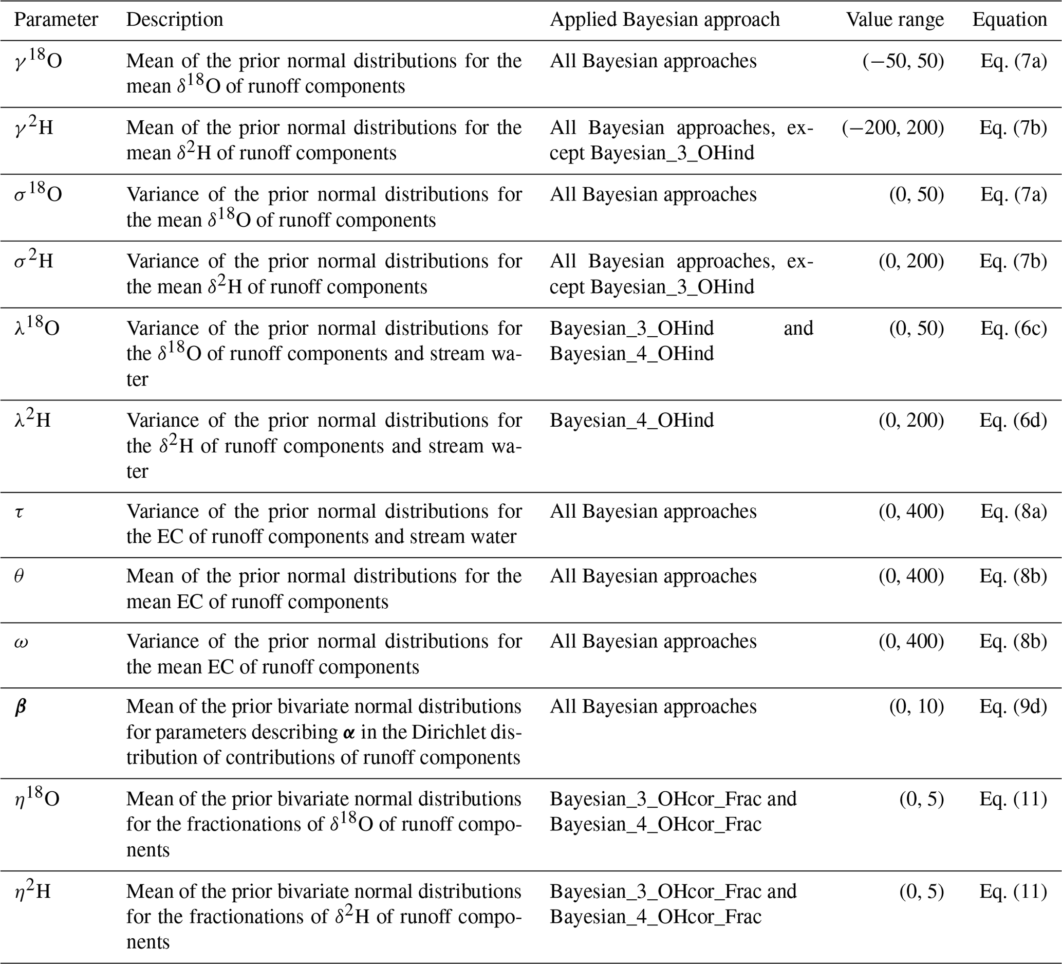
The Bayesian approaches applied for each season are summarized in Table 2. Similar to the EMMA, we apply a three-component Bayesian approach to all seasons and, additionally, a four-component Bayesian approach in the glacier melt season. The three-component Bayesian approach has two types. The Bayesian_3_OHcor approach considers the correlation between δ¹⁸O and δ²H, whereas the Bayesian_3_OHind approach assumes independence. The four-component Bayesian approach also has two types, namely the Bayesian_4_OHcor, which considers the correlation, and Bayesian_4_OHind, which assumes independence between δ¹⁸O and δ²H. A Kolmogorov–Smirnov test has been carried out for both isotope and EC tracers of all water sources before the application of Bayesian approaches. The tracer data of runoff components (i.e., rainfall, snowmelt, groundwater, and glacier melt) pass the normal distribution test at significance levels of p values > 0.3, apart from the EC data of glacier melt. The small glacier melt sample size for the EC measurement probably provides insufficient data for the distribution test. The tracer data of stream water also fail to pass the normal distributions test, which is partly caused by the extreme isotope and EC values (see Figs. S1a and S1b). Thus, the prior assumptions for the Bayesian approaches are listed (similar to Cable et al. 2011) as follows. In approaches considering the correlation between δ¹⁸O and δ²H, the prior distributions of δ¹⁸O and δ²H of runoff components are assumed to be bivariate normal distributions with means and precision matrix as μ¹⁸O, μ²H, and Ω, respectively (Eq. 6a). The precision matrix (Ω, i.e., the inverse of the covariance matrix) for the two isotopes is assumed to be Wishart prior (Eq. 6b). When assuming independence between δ¹⁸O and δ²H, the prior distributions of δ¹⁸O (δ²H) from runoff components are assumed to be normal distributions with means and variance of μ¹⁸O and λ¹⁸O (μ²H and λ²H; Eqs. 6c and d). The mean values of the isotopes of runoff components (i.e., μ¹⁸O and μ²H) are further estimated by independent normal priors (Eq. 7; Cable et al. 2011), which is assumed to consider the spatial variability of μ¹⁸O and μ²H.

where λ¹⁸O, γ¹⁸O, and σ¹⁸O (λ²H, γ²H and σ²H) are parameters used to describe the normal priors of δ¹⁸O and μ¹⁸O (δ²H and μ²H; see Table 3), which are estimated by likelihood observations. V is a 2 × 2 unit positive definite matrix, and “2” stands for the degree of freedom in the Wishart prior distribution.

The priors of EC values of runoff components are assumed to be normal distributions (Eq. 8a), with mean ε and variance τ. Similarly, the spatial variability of the mean EC values of runoff components (ε) is assumed to follow a normal distribution with mean θ and variance ω (Eq. 8b). Moreover, τ, θ and ω are parameters estimated by likelihood observations (Table 3).

The prior distributions of stream water are calculated in two steps. First, the prior distributions of δ¹⁸O, δ²H, and EC of stream water are assumed to be the same as those of runoff components in Eqs. (6) and (8a). Second, the mean isotopes (μ¹⁸O and μ²H) and EC (ε) of stream water are constrained by a mixing model (Eq. 9a and b), which estimates the isotope and EC mean values of stream water by multiplying the contribution of each runoff component (f_i) with the corresponding mean isotope and EC values of each runoff component (Eq. 9a).

where N is the number of runoff components. The contribution vector (f) is represented by a Dirichlet distribution with an index vector α (Eq. 9b), in which the sum of the contributions of all runoff components (∑f_i) equals one. The index vector α is estimated by two variable vectors, namely ρ and ψ (Eq. 9c), considering the temporal and spatial variability in the CRCs (Cable et al. 2011). ρ and ψ are assumed to be bivariate normal distribution with means and precision matrix β and Ω (Eq. 9d). Moreover, β is a parameter vector estimated by likelihood observations (Table 3).

The initial value ranges of parameters that need to be estimated in Eqs. (6)–(9) are summarized in Table 3. The posteriors of parameters describing the spatial variability of tracer signatures in Eqs. (7) and (8b) are first estimated by the mean tracer signatures of runoff components measured at different spatial locations. Parameters describing the overall variability of tracer signatures in Eqs. (6) and (8a) are then constrained by likelihood observations of tracer signatures from all water samples at different times and locations. The posterior distributions of CRCs (f) are estimated by Eq. (9), based on the posterior tracer signatures of runoff components and measured tracer signatures from stream water samples. The posteriors of parameters and contributions are estimated by the R software package RStan. We ran four parallel Markov chain Monte Carlo (MCMC) chains with 2000 iterations for each chain. The first 1000 iterations were discarded for warm-up, generating a total of 4 × 1000 samples for the calculation of the posterior distributions. Uncertainties are presented as the 5–95 percentile ranges from the iterative runs. The parameter values are assumed to follow uniform prior distributions within their value ranges to initialize the MCMC procedure.

Note that the four-component approaches (EMMA_4, Bayesian_4_OHcor, and Bayesian_4_OHind) are developed in our study to investigate the following two questions. (1) Is the EMMA able to quantify four runoff components just by using δ¹⁸O, δ²H, and EC? (2) Does the correlation between δ¹⁸O and δ²H help to reduce the uncertainty of the quantification of runoff components? The correlation between δ¹⁸O and δ²H is ignored in Bayesian_4_OHind. Thus, we used independent prior distributions for δ¹⁸O and δ²H of each water source. In Bayesian_4_OHcor, the posterior parameters describing the correlation between δ¹⁸O and δ²H vary among the water sources, thus providing a basis for the quantification of four runoff components using four mixing equations of tracer signatures, which is similar to Eq. (9).

3.3 Effects of the uncertainty of the meltwater sampling

Due to limited accessibility, meltwater samples are typically difficult to collect in high-elevation glacierized areas. Often only a few water samples are available to represent the tracer signatures of meltwater generated from the entire glacierized area. Hence, the representativeness of collected meltwater samples implies an additional uncertainty source in the hydrograph separation.

We thus define three virtual sampling scenarios to evaluate the effects of meltwater sampling on the EMMA and Bayesian mixing approaches. Scenario I is used to evaluate the effects of the sample size of meltwater in which four groups of meltwater sample are tested. The four sample groups have the same mean value and SD of δ¹⁸O or EC but different sample sizes. Mean and SD values of δ¹⁸O or EC are calculated for all available meltwater used samples in each group. Scenario II is used to evaluate the effects of the sampled mean value of δ¹⁸O (or EC) of meltwater. The four sample groups have the same sample size and SD but different mean values of δ¹⁸O (or EC). Scenario III is used to investigate the effects of SD values of sampled δ¹⁸O (or EC). The four sample groups have the same sample size and mean tracer signature but different SD values. Because meltwater is particularly difficult to collect, and is the dominant runoff component in the glacier melt season, we investigated the effects of the meltwater sampling uncertainty on the mixing approaches in this season. For the water samples of other runoff components and stream water, we used all the available measurements in the glacier melt season for the three virtual scenarios and kept the same sample characteristics. We only investigated the effects of sampling uncertainty in the glacier melt season because of the following reasons. (1) Runoff in the glacier melt season contributes the largest part to the annual runoff in our study basin. Accurate quantification of each runoff component in this season is extremely important for understanding the dynamics of water availability in the study area. (2) There are more meltwater samples available in this season (15 snowmelt samples and 23 glacier melt samples) than in the snowmelt season (only 15 snowmelt samples; Table 1), thus providing a good observation database for the investigation.

Table 1Tracer signatures measured from water samples in three seasons.

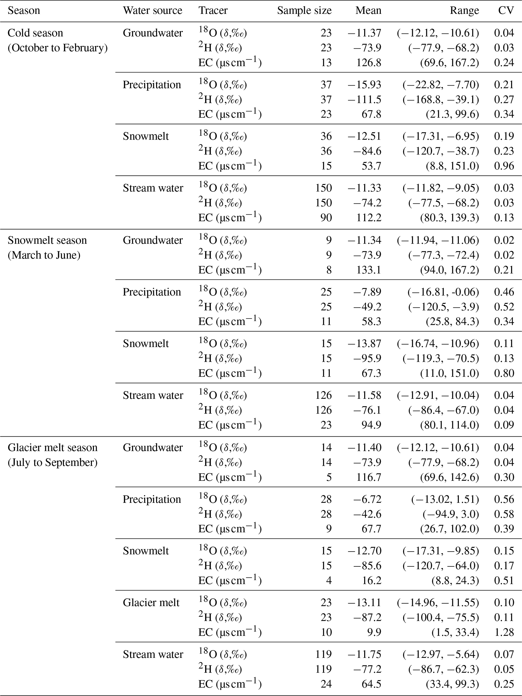
CV stands for coefficient of variation.

Download Print Version | Download XLSX

Table 2Mixing approaches applied for hydrograph separation in different seasons.

Download Print Version | Download XLSX

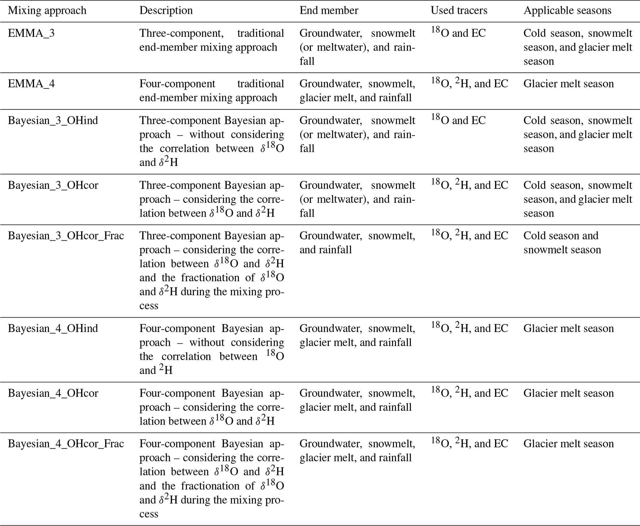
Table 3Parameters used for prior distributions in the Bayesian approaches.

Download Print Version | Download XLSX

3.4 Effects of water isotope fractionation on hydrograph separation

The water sources for runoff, such as rainfall and meltwater, are subject to evaporation before reaching the basin outlet – especially in summer. However, the isotopic composition of stream water was measured at the basin outlet, and the contributions of runoff components are also quantified for the total runoff at the basin outlet. After the long routing path from the sampled sites to the basin outlet, the isotopic compositions of rainfall and meltwater mixing at the basin outlet could be different from those measured at the sampled sites, which is caused by the evaporation fractionation effect. To consider the changes in the isotope signatures of water sources caused by the fractionation effect during the mixing process, we set up two modified Bayesian approaches, i.e., Bayesian_3_OHcor_Frac and Bayesian_4_OHcor_Frac (Table 2). The fractionation effect on the estimated CRCs is quantified by comparing two Bayesian scenarios. In the first scenario (using Bayesian_3_OHcor and Bayesian_4_OHcor), the isotopic compositions of water sources at the basin outlet are assumed to be the same as those measured from the sample sites even though the water sources have suffered evaporation before reaching the basin outlet (using Eqs. 6–9). In the second scenario (using Bayesian_3_OHcor_Frac and Bayesian_4_OHcor_Frac), the evaporation fractionation effect on the isotopic compositions of water sources is considered, and the mixing of water tracers for stream water is represented by Eq. (10). We modify the mean values in Eq. (9a) using the fractionation factors of ξ¹⁸O and ξ²H. The priors for ξ¹⁸O and ξ²H are assumed to be bivariate normal distributions in Eq. (11).

where η¹⁸O and η²H are parameters describing the mean values of the changes in isotopes caused by the fractionation effect. Ω is the inverse of the covariance matrix defined in Eq. (6b). The parameters in Eqs. (6)–(11) are then reestimated, using the MCMC procedure, by the measurements of tracer signatures. In particular, parameters describing the prior distributions of isotopic compositions at the sample sites in Eqs. (6) and (7) are estimated by the likelihood observations of isotope signatures of runoff components. The fractionation factors ξ¹⁸O and ξ²H are estimated by the likelihood observations of isotope signatures of stream water.

4.1 Seasonality of tracer signatures

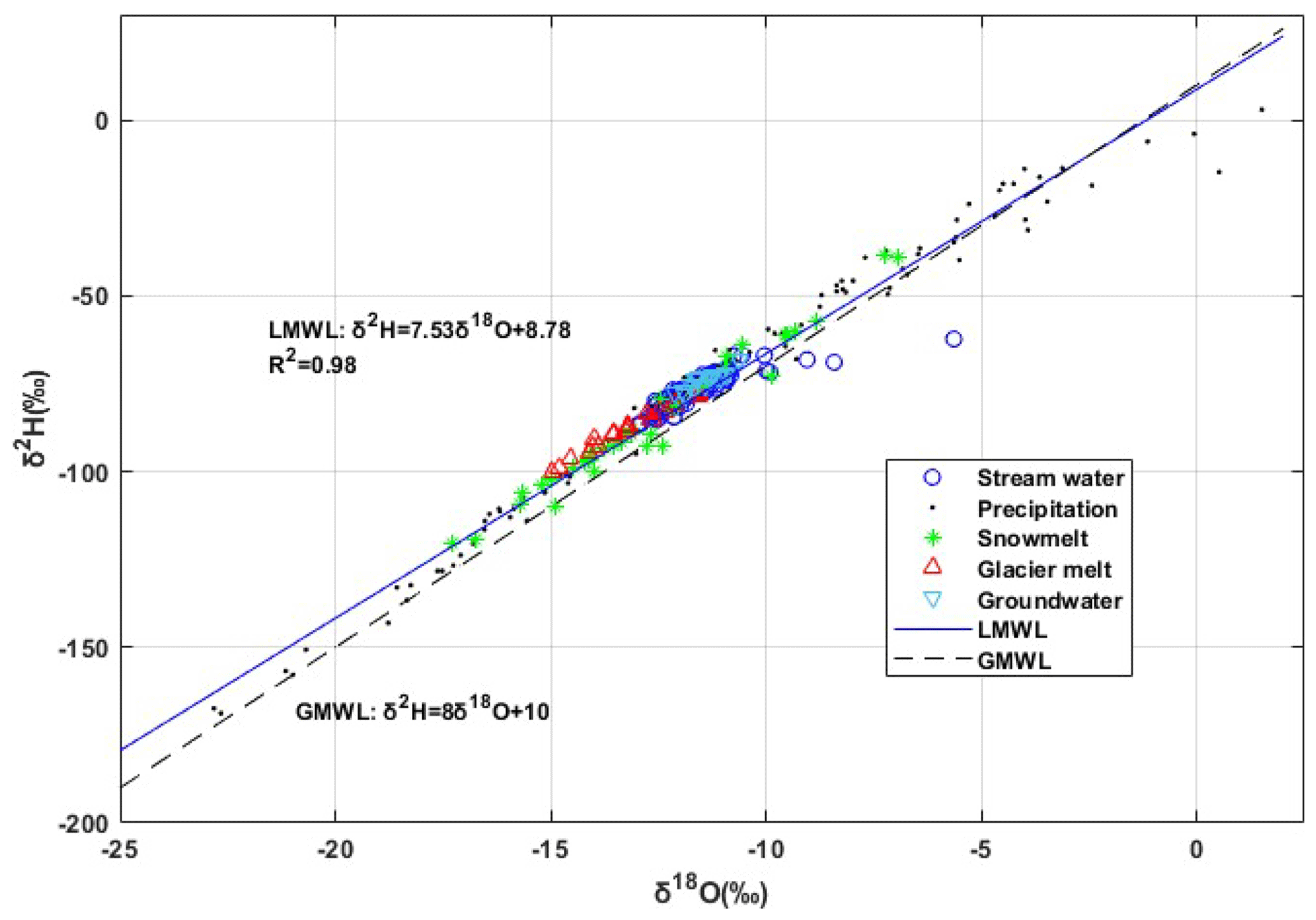
Tracer measurements from all the water samples are summarized in Table 1 and Fig. 2 (see also Fig. S1). The mean values in Table 1 indicate that precipitation is most depleted in heavy water isotopes (¹⁸O and ²H) among the water sources in the cold season. In the melt seasons, snow and glacier meltwater show the most depleted heavy isotopes. The EC values are highest in groundwater in all seasons and are followed by stream water and precipitation. Among the water sources, snowmelt and glacier melt tend to have the lowest EC values. Figure 2 shows that the slope of the local meteoric water line (LMWL) is lower than that of the global meteoric water line (GMWL). The δ¹⁸O of precipitation and snowmelt range from −22.82 ‰ to 1.51 ‰ and from −17.31 ‰ to −6.95 ‰, respectively. The isotopic composition of glacier meltwater is more depleted than that of groundwater and stream water. Stream water shows a similar isotopic composition to groundwater. Three samples from the stream water are far below the LMWL, which is likely caused by the evaporation effect.

Figure 2Isotope signatures of water samples from the three seasons in the Ala-Archa basin.

Download

CV values in Table 1 and boxplots in Fig. 3a–f show that the δ¹⁸O and δ²H of precipitation generally show the largest variability in all seasons, followed by the isotopes of snowmelt. Groundwater and stream water show the smallest CV values for δ¹⁸O in all three seasons. The stream water presents the lowest CV value for EC in all seasons, followed by the groundwater. The snowmelt EC shows high CV values in the snowmelt and glacier melt seasons, which may be attributed to variable dust conditions at the sampling locations (from the downstream gauge station to the upper glacier accumulation zone). The highest CV value of EC for glacier melt indicates large variability in the glacier melt samples (also see Fig. 3g–i). This is because the glacier melt water samples were collected from a rather clean location (EC value is only 1.5 µs cm⁻¹) and also a relatively dusty location (EC value is 33.4 µs cm⁻¹).

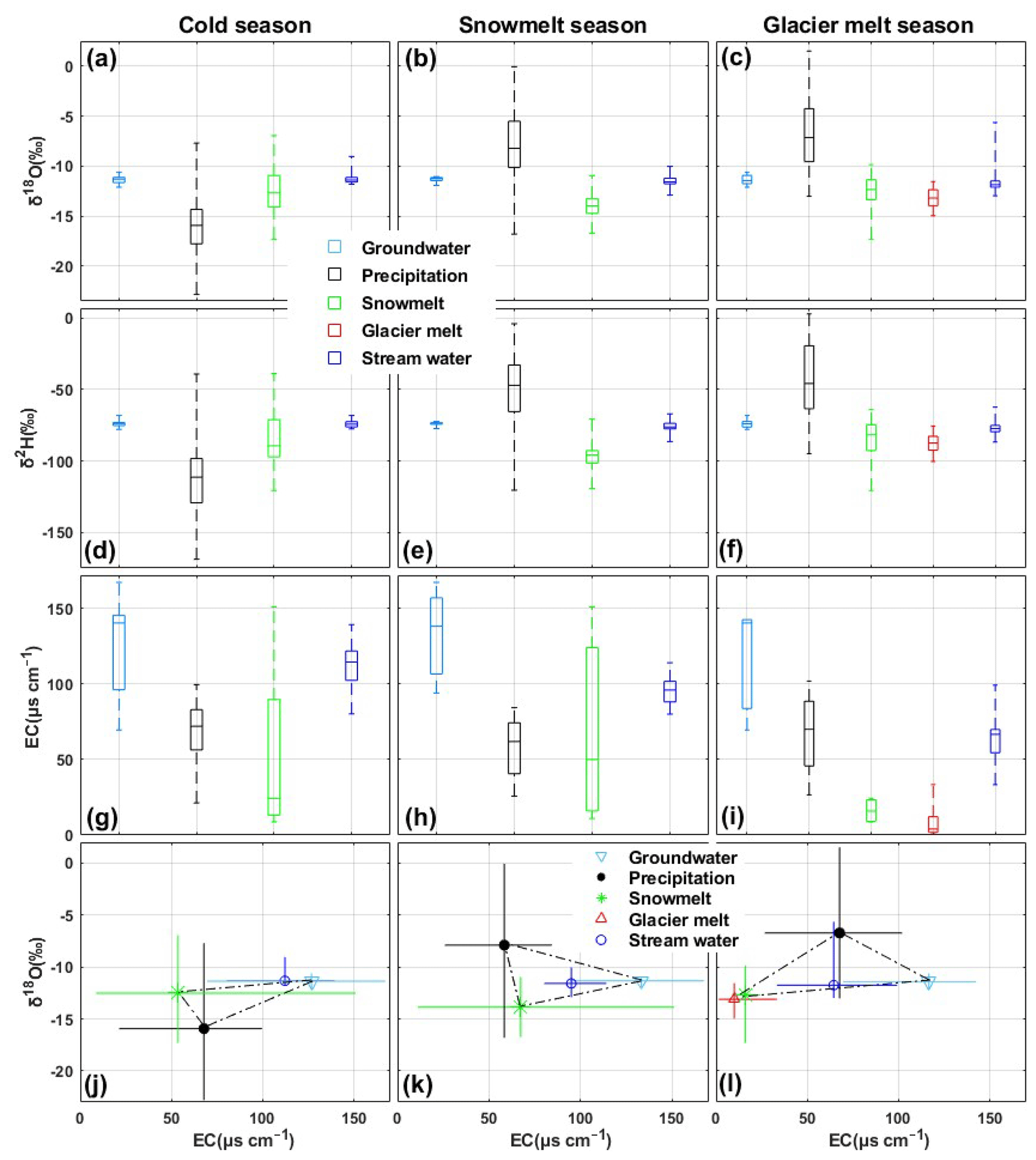
Figure 3(a–i) Boxplots of tracer signatures in three seasons. (j–l) δ¹⁸O–EC mixing space of the various water sources in the three seasons. The solid lines indicate the ranges of tracer signatures measured from water samples.

Download

For each water source, except groundwater, the tracer signatures show a significant seasonality (Table 1 and Fig. 3). In particular, the δ¹⁸O and δ²H of precipitation are most depleted in the cold season and reach the highest values in the glacier melt season, which is partly caused by the seasonality of the temperature. Stream water shows higher values of δ¹⁸O and EC in the cold season when groundwater dominates the streamflow and has lower values in the melt seasons when meltwater has a dominant contribution. Snowmelt has a lower EC value in the glacier melt season than in the cold and snowmelt seasons. In the cold and snowmelt seasons, some snowmelt samples also have EC values as low as those in the glacier melt season. The snow samples in the glacier melt season were only collected from the accumulation zone of the glacier, thus resulting in a small variability in the EC values. The snowpack in the accumulation zone is accumulated by fresh snow in the snowy period (summer-type accumulation glacier).This leads to low EC values in the snowmelt samples. The tracer signature of groundwater is relatively stable across the seasons.

Figure 3j–l show the δ¹⁸O–EC mixing space of runoff components in the three seasons. The ranges of solid lines indicate the minimum and maximum tracer values of individual water samples. In the cold season, the δ¹⁸O and EC values of stream water are very close to those of groundwater (Fig. 3j), whereas the snowmelt and precipitation tracer signatures show much more of a difference. These results indicate the dominance of groundwater on streamflow during the cold season. In the snowmelt and glacier melt seasons (Fig. 3k–l), the stream water samples are clearly located within the triangle formed by the samples of runoff components. The tracer signatures of glacier meltwater and snowmelt water are similar. The precipitation samples are further away from the stream water samples when compared to the meltwater and groundwater samples. The stream water samples are located nearly in the middle between the meltwater and groundwater samples. This indicates that the contribution of rainfall to total runoff is the smallest, and the contributions of meltwater and groundwater are similar in the melt seasons.

4.2 Contributions of runoff components estimated by the mixing approaches

Table 4 and Fig. 4 compare the CRCs estimated by the mixing approaches. In the cold season (Fig. 4a), the EMMA_3 estimated the mean contributions of groundwater and snowmelt as 83 % and 17 %, respectively. The mean contribution of rainfall is zero. The mean contributions of groundwater, snowmelt, and rainfall were estimated as 86 % (87 %), 13 % (12 %), and 1 % (1 %) by the Bayesian_3_OHind (Bayesian_3_OHcor) approach. As shown in Fig. 3j, the tracer signature of stream water in this season is close to that of groundwater, while obviously different from that of rainfall. Meanwhile, the stream water samples are outside of the triangle formed by the runoff components, leading to the zero contribution of the rainfall estimated by the EMMA_3.

Table 4Contributions of runoff components (CRCs) estimated by the different mixing approaches (percentage, %). The ranges (%) show the difference between the 95 % and 5 %  percentiles. SD values refer to the standard deviations.

Download Print Version | Download XLSX

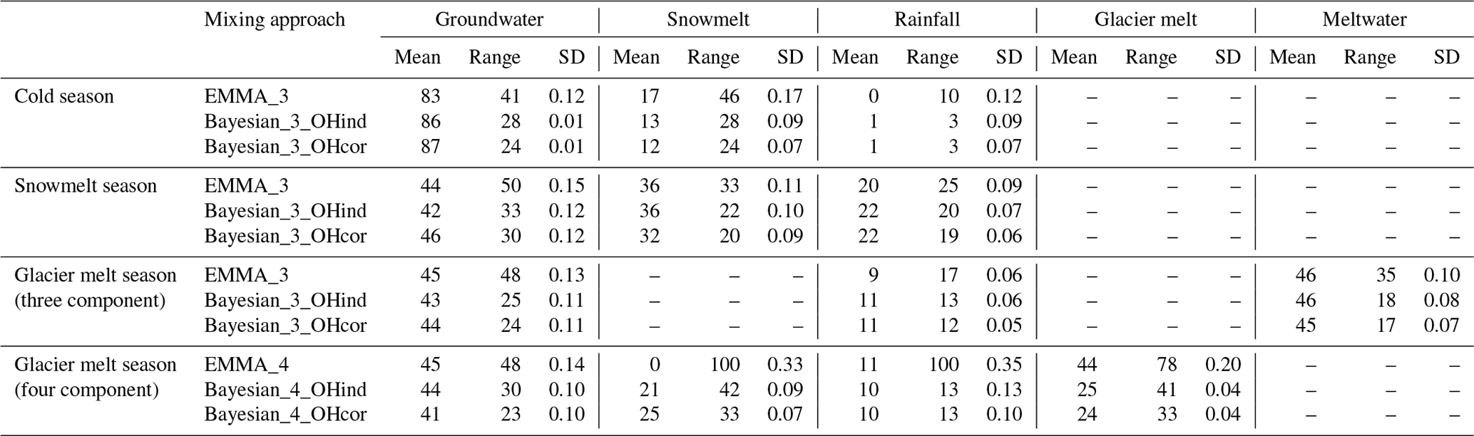
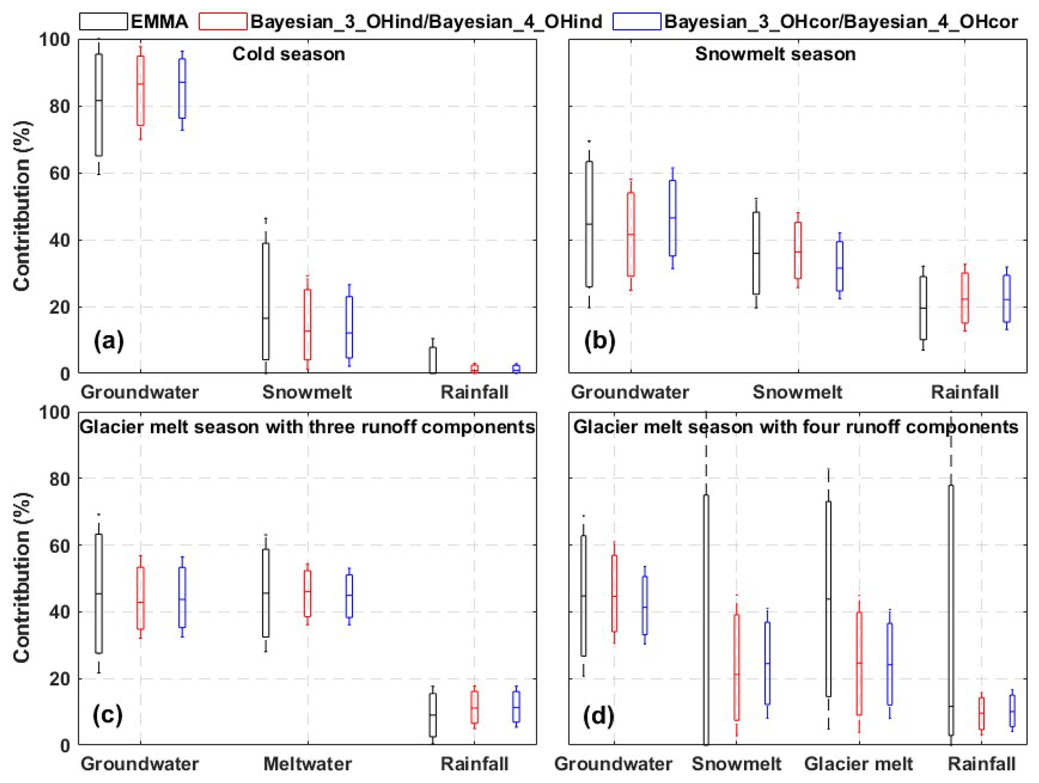
Figure 4Contributions of runoff components (CRCs) to total runoff estimated by different mixing approaches in three seasons. The Bayesian_3_OHind and Bayesian_3_OHcor were applied in the cold and melt seasons (a–c), and the Bayesian_4_OHind and Bayesian_4_OHcor were applied in the glacier melt season (d). The horizontal lines in the boxes refer to the median contributions, and the whiskers refer to the 95 % and 5 % percentiles.

Download

In the snowmelt season (Fig. 4b and Table 4), the EMMA_3 estimated the mean contributions of groundwater, rainfall, and snowmelt as 44 %, 36 %, and 20 %, respectively. The Bayesian_3_OHind estimated similar mean CRCs to EMMA_3, whereas the Bayesian_3_OHcor delivered a lower contribution of snowmelt (32 %). When treating the glacier melt and snowmelt as one end member (i.e., meltwater) in the glacier melt season (Fig. 4c), the EMMA_3 estimated the mean contributions of groundwater, meltwater, and rainfall as 45 %, 46 %, and 9 %, respectively. The Bayesian_3_OHind and Bayesian_3_OHcor estimated a lower contribution of groundwater (43–44 %) and a higher contribution of rainfall (11 %) compared to EMMA_3. The ranges and SD values of CRCs in Table 4 indicate the uncertainty of the estimates associated with the corresponding mixing approaches, showing that the EMMA_3, followed by Bayesian_3_OHind, produced the highest uncertainty of CRCs in all the three seasons. The Bayesian_3_OHcor reduced the uncertainty slightly when compared to Bayesian_3_OHind, as it benefits from the consideration of the correlation between δ¹⁸O and δ²H.

When treating glacier melt and snowmelt as two separate end members in the glacier melt seasons (Fig. 4d), the EMMA_4 failed to separate the hydrograph in the glacier melt season given the large uncertainty range in the contributions of snowmelt and rainfall (0–100 %). The tracer signatures of snow and glacier meltwater are rather close to each other, which violates the second assumption of the EMMA (see Sect. 3.1). In contrast, the Bayesian_4_OHcor and Bayesian_4_OHind estimated the shares of glacier melt and snowmelt as 25–24 % and 21–25 %, respectively. Considering the significant snow cover area in September in the study basin (He et al. 2018, 2019), the contribution of snowmelt in the glacier melt season should be higher than zero. Again, the Bayesian_4_OHcor produced smaller uncertainty ranges and SD values for the contributions of groundwater and meltwater compared to Bayesian_4_OHind and EMMA_4 (Table 4).

The posterior distributions of tracer signatures estimated by the Bayesian_4_OHcor in the glacier melt season are compared with the measured histograms of tracer signatures in Fig. 5. The Bayesian_4_OHcor generally produced similar distributions of water isotopes to the measured distributions in terms of the similar mean values. The estimated posterior SD values of the water isotopes are smaller than SD values of the measurements. This can be explained by the incorporation of prior distributions by the Bayesian_4_OHcor, which reduces the variability of water isotopes. The posterior SD values for EC of water sources are also smaller than the measured SD values. However, the posterior distributions of EC show some deviations from the distributions of measured EC (Fig. 5k–o), which is partly due to the very small sample sizes (see Table 1). The comparison between the posterior distributions of tracer signatures estimated by the Bayesian_3_OHcor and the measured distributions in the other seasons generally shows a similar behavior (not shown for brevity).

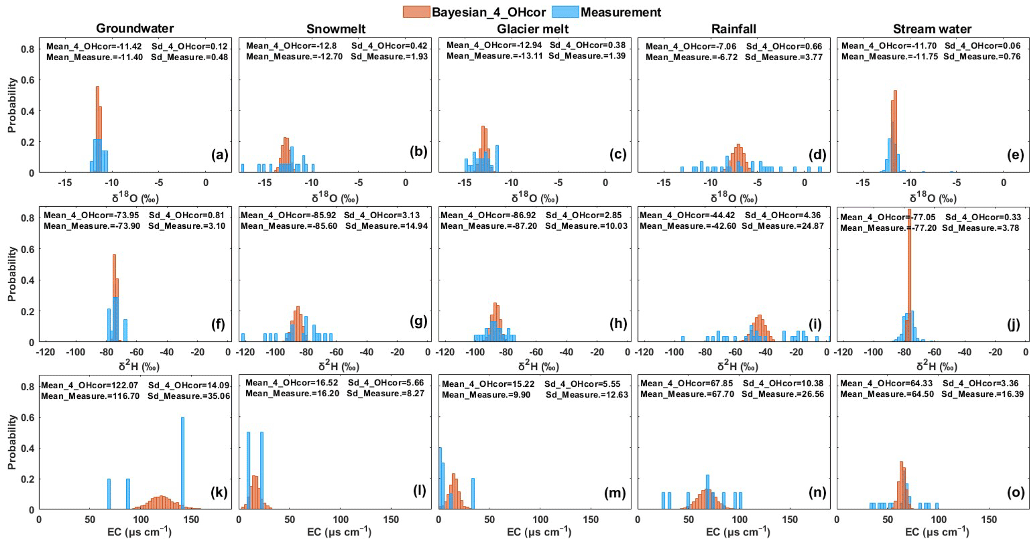
Figure 5Posterior distributions of tracer signatures estimated by the Bayesian_4_OHcor in the glacier melt season. Measurement refers to the distributions of tracer signatures from the water samples. (a–e) Distributions of δ¹⁸O; (f–j) distributions of δ²H; and (k–o) distributions of EC.

Download

The Bayesian_4_OHind estimated similar posterior distributions of tracer signatures to the Bayesian_4_OHcor (except the glacier melt isotopes; Fig. 6), with similar mean tracer values. It is noted that the Bayesian_4_OHcor estimated smaller SD values for most water sources compared to the Bayesian_4_OHind (e.g., Fig. 6f, g, i, and j). Benefiting from the prior information and the consideration of the correlation between δ¹⁸O and δ²H, the Bayesian_4_OHcor tended to produce the smallest variability in the posterior tracer signatures among all the mixing approaches (Figs. 5 and 6), thus resulting in the smallest uncertainty for CRCs (Fig. 4d). Figure 7 compares the correlation between δ¹⁸O and δ²H of the measured tracers and the posterior estimates by Bayesian approaches. The Bayesian_4_OHcor reproduced the correlation between δ¹⁸O and δ²H well in comparison to the measured data, whereas the Bayesian_4_OHind failed to capture the correlation.

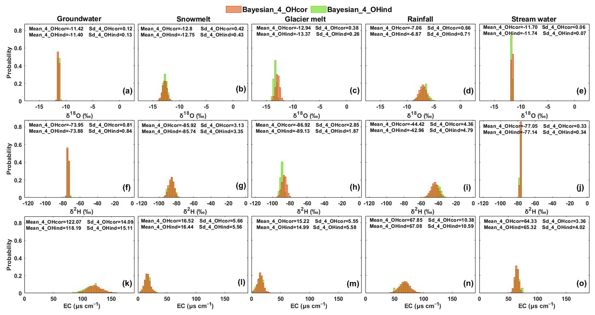
Figure 6Comparison of the posterior distributions of tracer signatures estimated by the Bayesian approaches with Bayesian_4_OHcor and without Bayesian_4_OHind considering the correlation between δ¹⁸O and δ²H in the glacier melt season.

Download

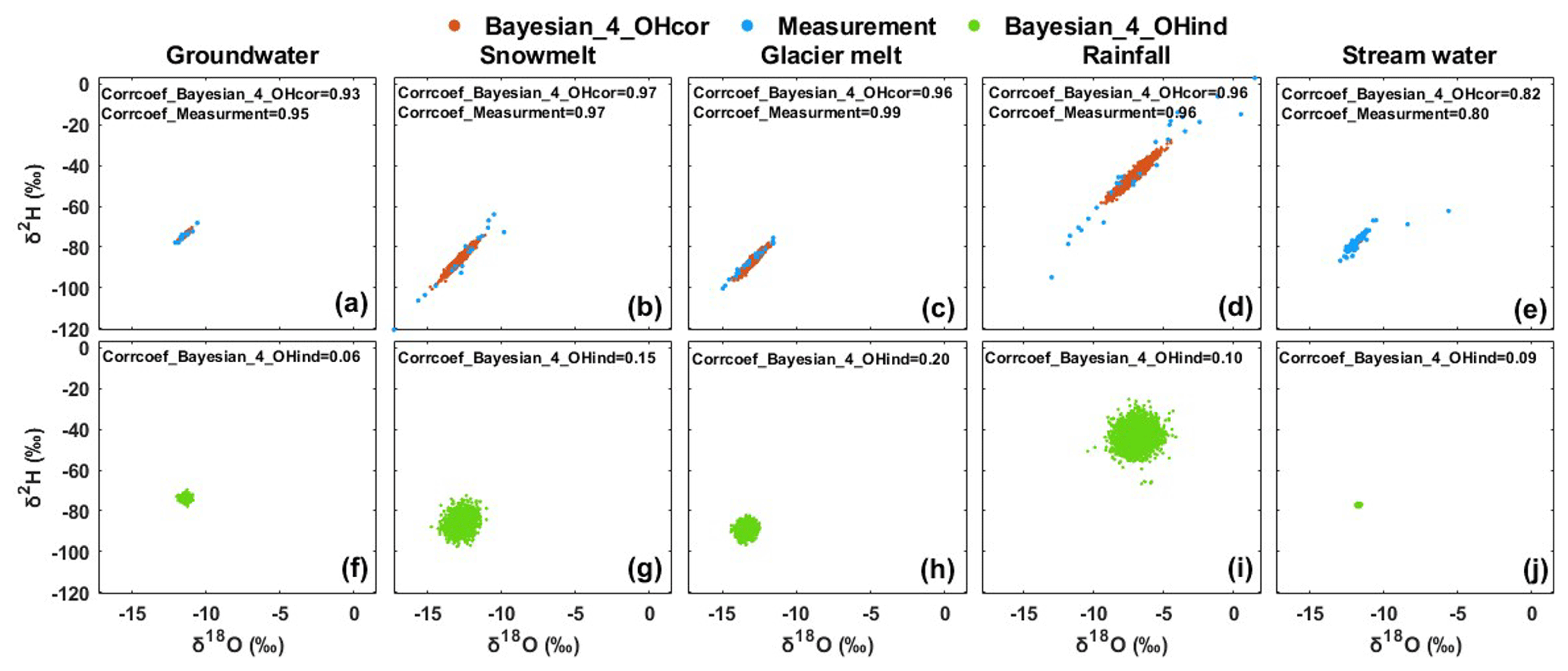
Figure 7Correlation between posterior δ¹⁸O and δ²H estimated by the Bayesian_4_OHcor and the Bayesian_4_OHind approaches in the glacier melt season.

Download

4.3 Uncertainty of hydrograph separation caused by sampling uncertainty of meltwater

Figure 8 shows the sensitivity of the Bayesian_3_OHcor and EMMA_3 approaches to the sampled δ¹⁸O of meltwater in the glacier melt season. The mean CRCs quantified by the two mixing approaches shows minor sensitivity to the sample size (Scenario I). However, the uncertainty ranges of contributions tend to decrease with increasing sample sizes, especially for EMMA_3. When assuming only two meltwater samples, the EMMA_3 resulted in very large uncertainty ranges (0–100 %; Fig. 8d), due to the very wide confidence interval for the SD at a sample size of two. The mean contributions of groundwater and meltwater estimated by the two mixing approaches decrease with the increasing mean δ¹⁸O of the adopted meltwater sample (Scenario II), while the estimated contribution of rainfall increases with the increasing mean δ¹⁸O (Fig. 8k). Variations in the mean CRCs quantified by EMMA_3 are larger than those estimated by the Bayesian_3_OHcor. Using EMMA_3, both the mean contributions of groundwater and meltwater declined by 9 % with the assumed increase of the mean δ¹⁸O (Fig. 8e and h), and the contribution of rainfall increased by 17 %. Using Bayesian_3_OHcor, the reduction of the contributions of groundwater and snowmelt are 4 % and 7 %, respectively, and the increase of the contribution of rainfall is only 11 % (Fig. 8k). In Scenario III, the uncertainty ranges of CRCs (especially for rainfall; Fig. 8l) increase with the increasing SD of the sampled δ¹⁸O. Again, the increases in the uncertainty ranges estimated by EMMA_3 tend to be larger than those estimated by the Bayesian_3_OHcor. The sensitivity of the mixing approaches to the sampled EC values of the meltwater are similar to the sensitivity of the sampled δ¹⁸O (not shown).

Figure 8Sensitivity of the CRCs estimates to the sample size (Scenario I), the mean (Scenario II), and standard deviation (Scenario III) of δ¹⁸O of meltwater samples in the glacier melt season. Red boxes show the contributions estimated by the Bayesian_3_OHcor, and the blue boxes refer to the contributions estimated by the EMMA_3.

Download

4.4 Effect of isotope fractionation on the hydrograph separation

The changes of δ¹⁸O caused by the fractionation effect (referring to ξ¹⁸O in Eq. 10) during the mixing process are estimated in Fig. 9a–c. The fractionation has the smallest effect on the δ¹⁸O of groundwater, while having the largest effect on the δ¹⁸O of rainfall. On average, the δ¹⁸O of rainfall increased by around 2.8 ‰ through fractionation in all the three seasons. The CRCs estimated by the Bayesian_3_OHcor_Frac and Bayesian_4_OHcor_Frac are compared with those estimated by the Bayesian_3_OHcor and Bayesian_4_OHcor in Fig. 9d–f, respectively. The mean contribution of groundwater estimated by the Bayesian_3_OHcor_Frac in the cold season is around 9 % lower than that estimated by the Bayesian_3_OHcor (Fig. 9d), while the mean contributions of snowmelt and rainfall are 3 % and 5 % higher, respectively. The reduction of the groundwater contribution should be attributed to the increased contributions of snowmelt and rainfall caused by the fractionation effect. In the snowmelt season, the mean contributions of groundwater and rainfall are 1 % and 7 % lower, respectively (Fig. 9e), while the mean contribution of snowmelt estimated by the Bayesian_3_OHcor_Frac is 8 % higher. In the glacier melt season, the mean contributions of groundwater and meltwater estimated by the Bayesian_4_OHcor_Frac are higher than those estimated by the Bayesian_4_OHcor (Fig. 9f) and are compensated by the 6 % lower contribution of rainfall.

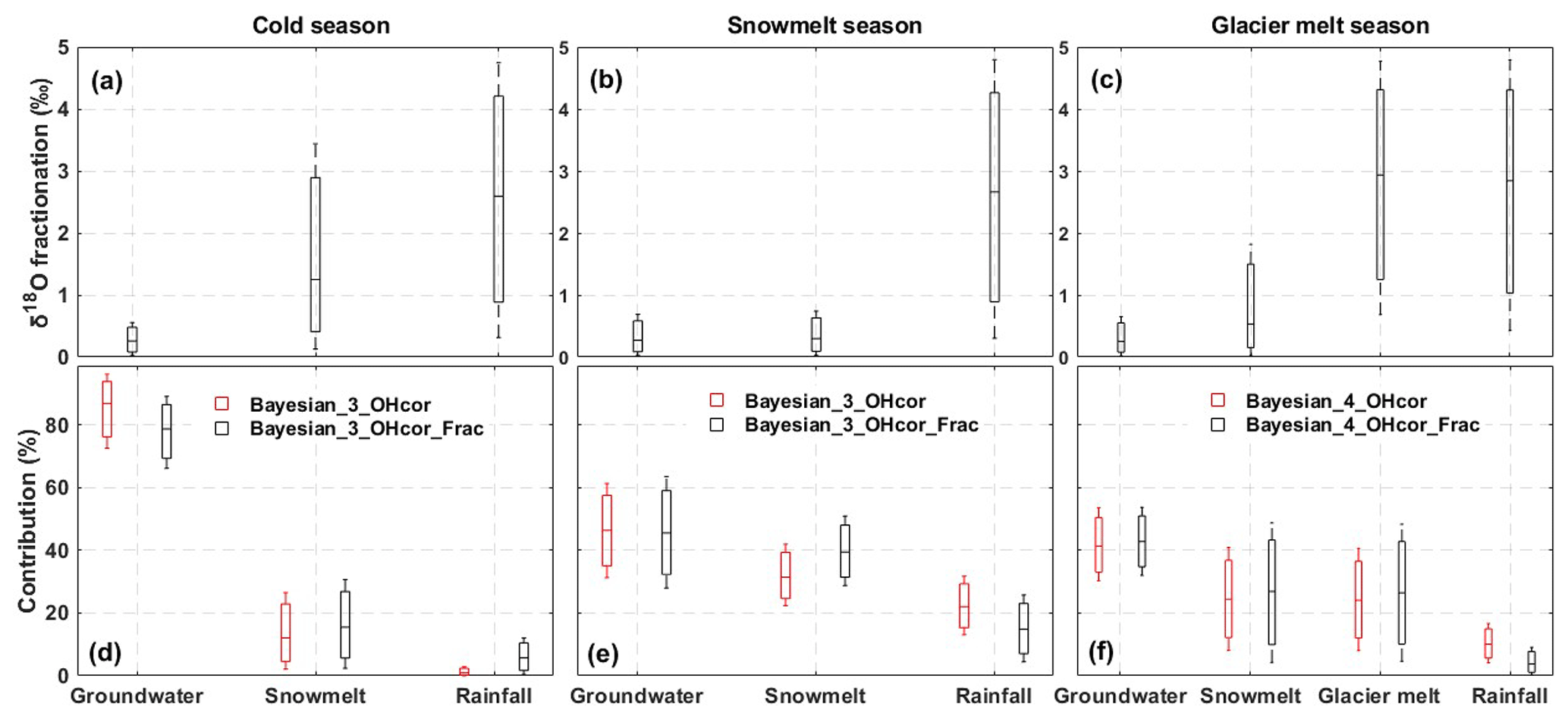
Figure 9Effects of isotope fractionation on the estimates of CRCs in the Bayesian approach for the three seasons. (a–c) Estimated changes in δ¹⁸O of runoff components caused by the fractionation effect; (d–e) CRCs estimated by the Bayesian_3_OHcor and the Bayesian_3_OHcor_Frac; and (f) CRCs estimated by the Bayesian_4_OHcor and the Bayesian_4_OHcor_Frac.

Download

The fractionation effect also produced visible changes in the posterior distributions of δ¹⁸O and δ²H of runoff components (Fig. 10 shows the example in the glacier melt season). The mean isotopic compositions of runoff components are increased by the fractionation effect. The SD values of the posterior isotopes estimated by the Bayesian_4_OHcor_Frac tend to be higher than those estimated by the Bayesian_4_OHcor due to the increased parameter space in the prior assumptions (Eq. 11), thus leading to the larger uncertainty ranges in the contributions of glacier melt and snowmelt (Fig. 9f). As expected, the estimates of posterior distributions of isotopic compositions of stream water are less sensitive to the fractionation effect of runoff components (Fig. 10e and j). The fractionation also has minor effects on the estimates of posterior distributions of EC values (Fig. 10k–o).

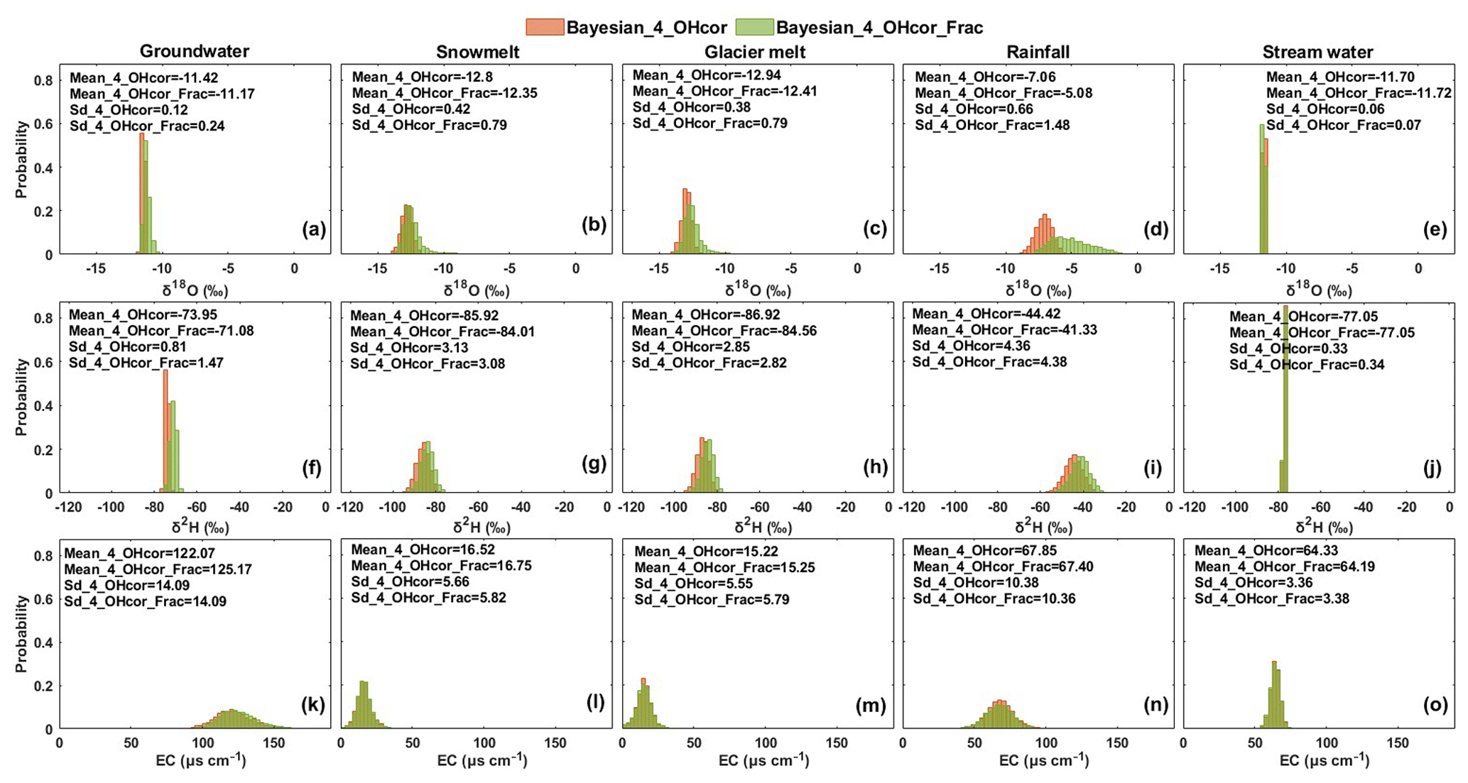
Figure 10Effects of isotope fractionation on the estimated posterior distributions of tracer signatures of water sources in the glacier melt season.

Download

5.1 Uncertainty of the contributions of runoff components

The EMMA estimated similar CRCs but with a larger uncertainty than the Bayesian approaches. The reasons for this are twofold. First, the EMMA estimated the uncertainty ranges of CRCs using the standard deviations (SD) of the measured tracer signatures. SD values are likely overestimated in this study due to the small sample sizes (i.e., low number of water samples) and thus represent the variability of the tracer signatures of the corresponding water sources across the basin insufficiently. Due to the limited accessibility of the sample sites caused by snow cover, the water samples of meltwater and groundwater are often collected sporadically. The small sample size and strong variability in sampled tracer signatures likely led to a large SD value in the measurement. Second, the EMMA assumes that the uncertainty associated with each water source is independent of the uncertainty of other water sources (Eq. 5), which increases the uncertainty ranges for CRCs.

In contrast, by updating the prior probability distributions, the Bayesian approaches estimated a smaller variability of tracer signatures in the posterior distributions when compared to the measured tracer signatures. The posterior distributions were sampled continuously from the assumed initial value ranges by the MCMC runs, thus reducing the sharp changes and yielding lower variability for the tracer signatures. Moreover, the uncertainty ranges for CRCs were quantified using Eqs. (6)–(10) instead of calculating independently as in the EMMA. Additionally, the assumed prior distributions of tracer signatures and the CRCs take the correlation between the tracer signatures and the dependence between the runoff components into account, thus resulting in smaller uncertainty ranges (Soulsby et al., 2003). For example, the Bayesian approaches that considered the correlation between δ¹⁸O and δ²H generally estimated smaller uncertainty ranges for CRCs compared to those that did not consider this correlation.

The Gaussian error propagation technique is only capable of considering the uncertainty of CRCs resulting from the variation in the tracer signatures (Uhlenbrook and Hoeg, 2003). The uncertainty of CRCs that originated from the sampling uncertainty of meltwater was then investigated in separate virtual sampling experiments. The EMMA produces large uncertainty ranges and SD values for CRCs in the glacier melt season when the meltwater sample size is rather small. The mean CRC quantified by the EMMA relies more heavily on the mean tracer values of the sampled meltwater, since the mean tracer values have been used directly in Eqs. (1)–(4), compared to the mean CRC estimated by the Bayesian approach.

The EMMA assumes that the tracer signature of each runoff component is constant during the mixing process; thus, it is unable to estimate the uncertainty of CRCs caused by the isotope fractionation effect. The virtual fractionation experiments, using the modified Bayesian approaches, show that the isotope fractionation could increase the contribution of snowmelt by 8 % and reduce the contribution of rainfall by 7 % in the snowmelt season. We assume that the mean CRCs estimated by the Bayesian approaches that consider the isotope fractionation are more plausible – despite the larger uncertainty ranges. Along the flow path from the source areas to the river channel, the isotopic compositions of meltwater and rainfall are likely increased by the evaporation fractionation effect – especially in the warm seasons. The increased isotopic compositions of meltwater and rainfall during the routing process need to be considered in the mixing approaches for hydrograph separation.

In general, the uncertainty of CRCs is visibly caused by the spatiotemporal variability in the tracer signatures, the water sampling uncertainty, and the isotope fractionation during the mixing process. The uncertainty caused by the water sampling of meltwater tends to be smaller than the uncertainty caused by the variations of the tracer signatures in both the EMMA and Bayesian mixing approaches. This is consistent with the findings that the SD values of the tracer measurements of water samples are the main uncertainty sources for the quantification of CRCs (Schmieder et al., 2016, 2018). The Bayesian approach tends to be superior for narrowing the variability of posterior tracer signatures benefitting from the prior assumptions and the consideration of the dependence between tracer signatures and runoff components when compared to EMMA.

5.2 Limitations

The representativeness of the water samples is one of the limitations of this study. The groundwater was only sampled from a single spring located at an elevation of 2400 $\mathrm{m}\mathrm{a}.\mathrm{s}.\mathrm{l}.$, which is rather close to the average altitude of the entire river network in the study basin (2530 $\mathrm{m}\mathrm{a}.\mathrm{s}.\mathrm{l}.$). We thus assume that the measured isotopic composition of the spring water represents the mean isotopic composition of the groundwater feeding the river in the basin (see also He et al., 2019). Collecting samples from a few springs to represent the groundwater end member has been proposed before (e.g., Ohlanders et al., 2013 and Mark and McKenzie, 2007), as the accessibility and availability of more potential springs are hampered. Again, for the snow and glacier meltwater samples, we assume that meltwater occurring at similar elevations has similar tracer signatures (He et al., 2019). The sampled elevation ranges from 1580 to 4050 $\mathrm{m}\mathrm{a}.\mathrm{s}.\mathrm{l}.$ and matches the elevation range where meltwater mainly occurs in the basin (from 1580 to 3950 $\mathrm{m}\mathrm{a}.\mathrm{s}.\mathrm{l}.$). Considering that the isotopic compositions of meltwater are particularly dependent on the elevation, the sampled meltwater could represent meltwater that originated from the primary melting locations in the entire basin. The sampled sites thus bear the potential to provide tracer signatures of the major meltwater generated in the basin.

We split the entire sampling period (from 2012 to 2017) into three seasons, i.e., cold season, snowmelt season, and glacier melt season, due to the low availability of the water samples in each year. By concentrating water samples in the three seasons, we increased the sample sizes of each runoff component for each season, thus increasing the ability of water samples to represent the spatiotemporal variability of seasonal tracer signatures. We used all available groundwater and snowmelt samples from the three seasons for hydrograph separation in the cold season due to the rather low number of samples collected in the cold season. This likely leads to overestimated contributions from groundwater and snowmelt in the cold season. However, the overestimation of the groundwater contribution is probably small because the tracer signatures of groundwater generally show small seasonal variability. The estimated contributions of snowmelt in the cold season are a bit higher than the contribution modeled by He et al (2018) during winter months of December, January, and February; these are still reasonable when considering that the cold season includes October and November when the snow is more prone to melting.

The assumptions of the mixing approaches lead to another limitation of this study. The EMMA assumes the tracer signatures of water sources are constant during the mixing process, which is a common assumption for the practical application of EMMA. It thus fails to consider the uncertainty originating from the changes of tracer signatures. In the Bayesian approach, we assumed normal prior distributions for the tracer signatures of water sources and Dirichlet prior distribution for the CRCs based on the literature (Cable et al., 2011). To refine the description of the temporal and spatial variability of the CRCs in the Dirichlet distribution, more hydrological data relating to the runoff processes in the basin are required. We acknowledge that the estimated CRCs could be strongly affected by the assumptions of prior distributions. However, testing the effects of the prior assumptions goes beyond the scope of this study. We assume that collecting more water samples from various locations and at different times for each water source could improve the estimation of tracer signature distributions.