2.1 Extracting seasonal components from time series

2.2 Linear reservoir theory

The derivations presented here all rely on the assumption of a linear time-invariant system (see e.g. Dooge, 1973, for an overview of linear systems theory). This implies that forcings of different wavelengths are not influencing each other. This is invalid for most real systems, yet the assumption of linearity is still widely made, as it can yield useful insights.

A linear reservoir is described by

where Q (mm d⁻¹) is the outflow from the reservoir, S is storage (mm), and τ (d) is a time constant describing how fast (slow) the reservoir responds. Conservation of mass requires

where Q_in is the inflow to the reservoir.

2.2.1 Periodic forcing of a linear reservoir

If we approximate the seasonal input to a linear reservoir by a sine wave of period T (e.g. 1 year), we can combine Eqs. (1), (5), and (6) to obtain

$$\begin{array}{}\text{(7)}& {\displaystyle \frac{\mathrm{d}{Q}_{\sin }}{\mathrm{d}t}}={\displaystyle \frac{\stackrel{\mathrm{‾}}{F}}{\mathit{\tau }}}\left(\mathrm{1}+{\mathit{\delta }}_F\sin \left({\displaystyle \frac{\mathrm{2}\mathit{\pi }}{T}}t+{\mathit{\varphi }}_F\right)\right)-{\displaystyle \frac{Q_{\sin }}{\mathit{\tau }}}.\end{array}$$

We might neglect the (initial) phase if we choose a starting time t that is aligned with the seasonal forcing component (ϕ_F=0). It can be shown that the steady-state response of a linear reservoir to a sinusoidal input signal is a damped and phase-shifted version of the input signal (see Sect. S1.1 for a more detailed derivation; or Eriksson, 1971; Peters et al., 2003).

$$\begin{array}{}\text{(8)}& Q_{\sin }\left(t\right)=\stackrel{\mathrm{‾}}{F}\left(\mathrm{1}+{\mathit{\delta }}_{F}A\sin \left({\displaystyle \frac{\mathrm{2}\mathit{\pi }}{T}}t+\mathit{\varphi }\right)\right),\end{array}$$

where A is the amplitude ratio and ϕ is the phase shift induced by a single linear reservoir.

$$\begin{array}{}\text{(9)}& {\displaystyle }& {\displaystyle }A={\displaystyle \frac{\mathrm{1}}{\sqrt{\mathrm{1}+{\left(\mathrm{2}\mathit{\pi }\frac{\mathit{\tau }}{T}\right)}^{\mathrm{2}}}}}\text{(10)}& {\displaystyle }& {\displaystyle }\mathit{\varphi }=\arccos \left({\displaystyle \frac{\mathrm{1}}{\sqrt{\mathrm{1}+{\left(\mathrm{2}\mathit{\pi }\frac{\mathit{\tau }}{T}\right)}^{\mathrm{2}}}}}\right)=\arccos \left(A\right).\end{array}$$

We can rewrite Eq. (8) as follows:

$$\begin{array}{}\text{(11)}& Q\left(t\right)=\stackrel{\mathrm{‾}}{Q}\left(\mathrm{1}+{\mathit{\delta }}_Q\sin \left({\displaystyle \frac{\mathrm{2}\mathit{\pi }}{T}}t+\mathit{\varphi }\right)\right).\end{array}$$

In a steady-state mass-conserving system, the mean of the output should equal the mean of the input. If the means obtained from data are different, either the forcing term is inaccurate (e.g. due to differences between actual and potential evapotranspiration) or the streamflow term is inaccurate (e.g. due to other losses or gains). The product of input amplitude and amplitude ratio equals the output amplitude (${\mathit{\delta }}_F\stackrel{\mathrm{‾}}{F}A={\mathit{\delta }}_Q\stackrel{\mathrm{‾}}{Q}$).

From Eqs. (9) and (10), we can see that the amplitude ratio and the phase shift are given by A and arccos(A), respectively. Since A is fully defined by the ratio between τ and T and T is usually known (e.g. 1 year), we can theoretically use A to determine the time constant τ of the reservoir. This requires the identification of both the seasonal components of the input and output signal of that period (see Sect. 2.1) and assumes the system to behave as a single linear reservoir. In theory, we could also apply the theory to periods other than 1 year, but for the reasons stated above we only investigate the annual period.

The amplitude ratio A and the phase shift arccos(A) can be plotted against each other for various values of τ as shown in Fig. 1. This results in a characteristic curve which captures the response of all single linear reservoirs. Different time constants τ (as proportions of the period; here 1 year) lead to different positions on the curve. For very fast reservoirs, the phase shift is close to 0 d, and the amplitude ratio is close to unity (that is, the signal is not attenuated at all). For very slow reservoirs, the signal is phase shifted up to 91 days, and the amplitude ratio approaches 0. The maximum phase shift of about 91 days corresponds to a quarter of a period (90^∘). Mathematically, this can be explained by Eq. (10), as the arccosine of a quantity between 0 and unity (such as A) ranges between 0 and 90^∘.

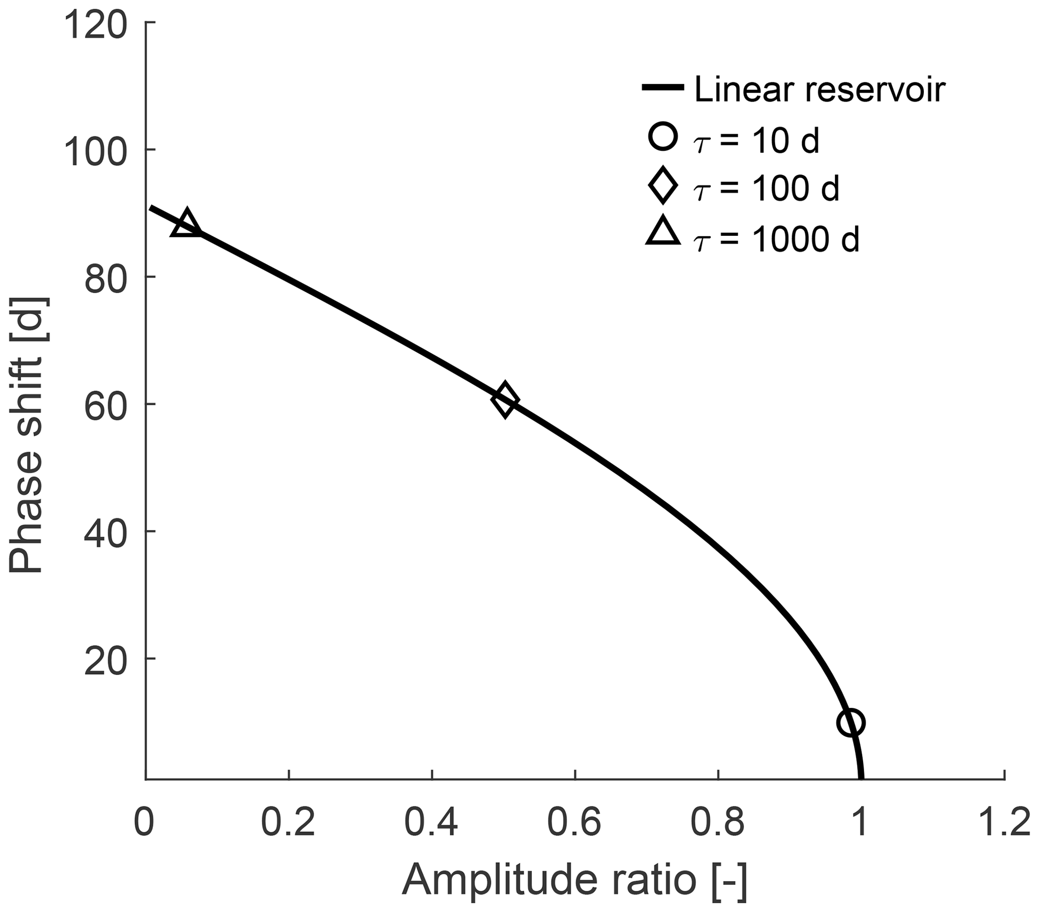
Figure 1Amplitude ratio against phase shift for a single linear reservoir for varying time constants τ. Three example time constants are indicated by the symbols.

Download

Note the similarity of Fig. 1 to Fig. 3c in Kirchner (2016), which shows the relationship between amplitude ratio and phase shift for gamma-distributed catchment transit time distributions. An exponential transit time distribution (a special case of the gamma distribution) corresponds to a linear reservoir describing the velocity of particles. Similarly, a linear reservoir describing the impulse response (the linear reservoir from Eq. 5), i.e. the celerity of the incoming wave of hydraulic potential, corresponds to an exponential response time distribution or an exponential unit hydrograph (cf. Eriksson, 1971; Dooge, 1973).

2.2.3 Linear reservoirs in series

Linear reservoirs in series can be conceptualised as follows. Every outflow is the inflow to the next reservoir. Hence, if the ith reservoir has a time constant τ_i, the amplitude ratios A_i are multiplied, and the phase shifts ϕ_i are added (see Sect. S1.2 for a more detailed derivation).

$$\begin{array}{}\text{(12)}& {\displaystyle }& {\displaystyle }{A}_{\mathrm{tot}}=\prod _{i=\mathrm{1}}^n{A}_i\text{(13)}& {\displaystyle }& {\displaystyle }{\mathit{\varphi }}_{\mathrm{tot}}=\sum _{i=\mathrm{1}}^n{\mathit{\varphi }}_i=\sum _{i=\mathrm{1}}^n\arccos \left(A_i\right)\end{array}$$

Figure 2 shows the amplitude ratio plotted against the phase shift similar to Fig. 1, but now for two linear reservoirs it includes two linear reservoirs in series. The different lines are examples with fixed time constants of the first reservoir. They all start from the black line (from the points marked by the symbols in Fig. 1), the characteristic curve for a single linear reservoir, which is the lower limit. Then, as the time constant of the second reservoirs increases, the lines “move” left and upwards, which corresponds to a decrease in amplitude ratio and an increase in phase shift. For example, the red line (τ₁=10 d) starts out with a phase shift of about 10 d and ends at a phase shift of about 101 d, which is an increase of about 91 d, the maximum phase shift of the second reservoir. The lines cross each other as we allow τ₂ to be larger than τ₁. This implies that sometimes a faster reservoir is followed by a slower one, and sometimes a slower reservoir is followed by a faster one. The grey shaded area contains all possible combinations for two reservoirs in series. The lower limit is a single linear reservoir. The upper limit corresponds to two reservoirs with the same time constant (a two-reservoir Nash cascade), which equals a gamma distribution with a shape parameter equal to 2 (Nash, 1957).

Figure 2Amplitude ratio against phase shift for two linear reservoirs in series. Each line corresponds to a fixed time constant for the first reservoir (τ₁), while the time constant of the second reservoir varies ($\mathrm{1}\mathrm{d}\le {\mathit{\tau }}_{\mathrm{2}}\le \mathrm{10}\mathrm{000}$ d; it is increasing from right to left). The black line indicates a single linear reservoir (the lower boundary). The grey line indicates the upper boundary where τ₁=τ₂. The shaded area contains all possible combinations of amplitude ratio and phase shift for two linear reservoirs in series.

Download

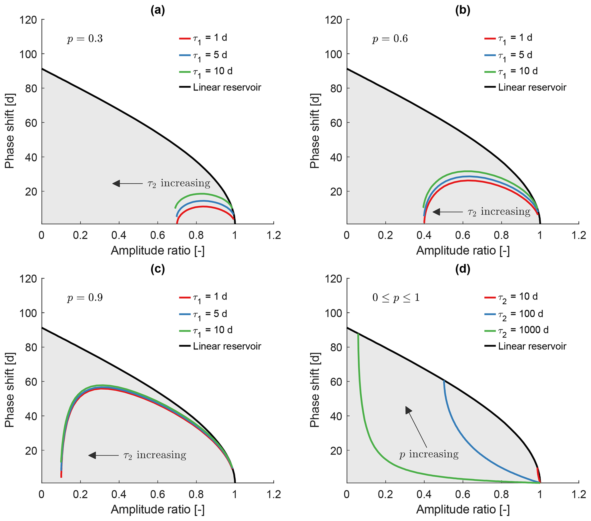
Figure 3Amplitude ratio against phase shift for two linear reservoirs in parallel. (a) Each line has a fixed time constant for the first reservoir (τ₁), while the time constant of the second reservoir varies ($\mathrm{10}\mathrm{d}\le {\mathit{\tau }}_{\mathrm{2}}\le \mathrm{10}\mathrm{000}$ d; it is increasing from right to left). The fraction p going into the second reservoir is 0.3. (b) Same as (a) with p=0.6. (c) Same as (a) with p=0.9. (d) Each line has a fixed time constant for the first reservoir (τ₁=1 d) and for the second reservoir (τ₂). The fraction p going into the second reservoir is varied (it is increasing from right to left). The shaded area contains all the possible combinations of amplitude ratio and phase shift for two linear reservoirs in parallel.

Download

2.3 Seasonal signatures as a diagnostic tool for evaluating hydrological models

We use two conceptual rainfall–runoff models and we test whether the seasonal signatures can be used as a diagnostic tool to assess model performance (Gupta et al., 2008). In particular, we test whether the models are capable of reproducing the range of observed signatures without calibrating them to streamflow data (cf. Vogel and Sankarasubramanian, 2003). This modelling experiment is intended to test whether the proposed signatures have the potential to be a useful additional source of information in model building and evaluation. We do not intend (or suggest) that the presented evaluation approach can replace existing model evaluation methods. We limit the analysis to 2 models and 40 catchments to keep the computational demand manageable. We also limit the model evaluation to catchments in the UK, as the seasonal signatures are unreliable in arid catchments (see Sect. 5). The subset of catchments is described in Sects. 3 and S3.1.

The first model is the IHACRES model. It is conceptually relatively similar to the considerations in Sect. 2. It has a soil moisture store (non-linear deficit store) and two parallel linear stores for fast flow and for slow flow (Croke and Jakeman, 2004). It has been used in many modelling studies in Australia (Post and Jakeman, 1999) and also in the UK (Sefton and Howarth, 1998). The second model is the GR4J model. It also has a parallel flow structure, but the internal parametrisation is different. It contains more non-linearities, and it has fixed internal parameters. Additionally, it has a groundwater exchange parameter aimed at representing inter-catchment groundwater flows. It has been used in many modelling studies in France (Perrin et al., 2003), in the UK (Smith et al., 2019; Harrigan et al., 2018b), and in the US (Oudin et al., 2018). We use the implementations of the two models in the Modular Assessment of Rainfall-Runoff Models Toolbox (MARRMoT) v1.2 (Knoben et al., 2019a), a MATLAB toolbox containing many hydrological models aimed at model comparison studies. The pure delay function in the MARRMoT implementation of IHACRES is set to 0, making it (conceptually, not necessarily numerically) equal to the version used by Croke and Jakeman (2004). In our modelling experiment, IHACRES has therefore six parameters, and GR4J has four parameters. Detailed information on the parameter ranges and on model warm-up periods can be found in Sect. S3.

To test which ranges of seasonal signatures the two models can reproduce, we run a Monte Carlo sampling experiment. We sample parameter sets for both models using Latin hypercube sampling, an efficient sampling method (Cheng and Druzdzel, 2000) that assumes uniform prior parameter distributions. With the parameter sets obtained, we run both models for each of the 40 catchments; i.e. we use the same parameter sets for each catchment. To test for robustness, we sample an increasing number of parameter sets (20 000 parameter sets are considered sufficient; see Sect. S3.2 for more information). We then use the modelled streamflow time series to calculate three hydrological signatures per parameter set: the two seasonal signatures presented here and the baseflow index. The resulting modelled signatures are compared to observed signatures and explored in a rather general way, as we want to examine what the models can do without actually calibrating them to streamflow data (cf. Vogel and Sankarasubramanian, 2003). That is, we are not interested in finding the “best” parameter set but in whether a certain model (given certain parameter ranges) is generally capable of reproducing the signatures we observe.

3.1 Data sources

We use catchment data from the UK and the US. The data for the UK are obtained from different sources. Daily streamflow data, catchment characteristics, and catchment boundaries are obtained from the National River Flow Archive (NRFA; National River Flow Archive, 2019); precipitation data are from the UK Centre for Ecology & Hydrology's gridded estimates of daily and monthly areal rainfall for the UK (CEH-GEAR; Tanguy et al., 2016); and potential evapotranspiration data are from the climate hydrology and ecology research support system potential evapotranspiration dataset for Great Britain (CHESS-PE; Robinson et al., 2016). For the model evaluation we select catchments that are part of the UK Benchmark Network (UKBN; Harrigan et al., 2018a), which describes catchments in the UK that are near-natural. The subset of catchments is chosen to be representative of the UK; details are shown in Sect. S3.1. The data for the US are obtained from the Catchment Attributes and Meteorology for Large-sample Studies (CAMELS) dataset (Newman et al., 2015; Addor et al., 2017a). CAMELS includes daily precipitation, potential evapotranspiration (we use Daily Surface Weather and Climatological Summaries forcing data; Daymet) and streamflow data as well as a wide range of catchment attributes for 671 catchments in the contiguous US. We trim the daily data to contain only full water years (starting 1 October), and we analyse data from 1989 to 2009. We also remove catchments with missing records during that time period. While we need to pick a start date for the analysis, this date does not influence the results (e.g. using 1 January as the starting date would result in the same phase shift).

3.2 Hydrological signatures and catchment attributes

We calculate different hydrological signatures, and we use different catchment attributes, all summarised in Table 1. The climate indices from Knoben et al. (2018) are based on monthly averages, and they need to be interpreted as follows. A moisture index I_m of 1 indicates the most humid (energy-limited) catchments; a moisture index of −1 indicates the most arid (water-limited) catchments. A moisture index seasonality I_m,r of 0 indicates catchments where the climate stays constant throughout the year; a moisture index seasonality of 2 indicates catchments where the climate switches between fully arid and fully humid within the year.

Table 1Hydrological signatures and catchment attributes used in this study.

^a Should in theory be smaller than unity. ^b Should theoretically always be positive and in practice be smaller than 1 year. Further discussions on the possible ranges of the seasonal signatures can be found in the text. PROPWET: PROPortion of time soils are WET.

Download Print Version | Download XLSX

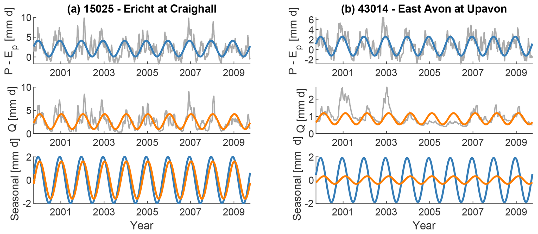
Figure 4Climate input (P−E_p; blue) and catchment output (Q; orange) for two example catchments in the UK and their respective seasonal components. The time series are smoothed using a 30 d moving mean. The Ericht is a rather responsive catchment (BFI = 0.47), while the East Avon has a large baseflow component (BFI = 0.89). Note that for the bottom plots (“Seasonal”) the mean values of the sine curves are set to 0.

Download

4.1 Extracting seasonal components from time series

First, we extract seasonal components from P−E_p (forcing) and Q (streamflow) for all catchments. The resulting sine wave parameters are then used to calculate the amplitude ratios (Eq. 3) and phase shifts (Eq. 4), respectively. Figure 4 shows P−E_p and Q for two catchments alongside their seasonal (sinusoidal) components. Both catchments experience a similar forcing, but their response is very different. The Ericht at Craighall, a rather responsive catchment, shows a seasonal streamflow component that is very similar to the seasonal forcing component. In contrast, the East Avon at Upavon, a groundwater-dominated catchment, shows a strongly attenuated seasonal streamflow component. For our seasonal signatures this would mean (a) that the responsive catchment has a high amplitude ratio (i.e. the streamflow amplitude is almost as large as the forcing amplitude, while the groundwater-dominated catchment has a low amplitude ratio) and (b) that the responsive catchment has a small phase shift (i.e. it responds quickly to the seasonal forcing, while the groundwater-dominated catchment has a large phase shift).

4.2 Seasonal signatures of observed catchment data

To visualise the seasonal signatures, we plot the amplitude ratios and phase shifts in a similar way as in Figs. 1–3. This is shown in Fig. 5a for all UK catchments. These include catchments with human influences, such as groundwater abstractions, man-made reservoirs, or water transfers. The overall pattern in Fig. 5a is very similar to the pattern using benchmark catchments alone (grey dots). We therefore use all of the catchments, noting that a few catchments might be unsuitable for individual analyses.

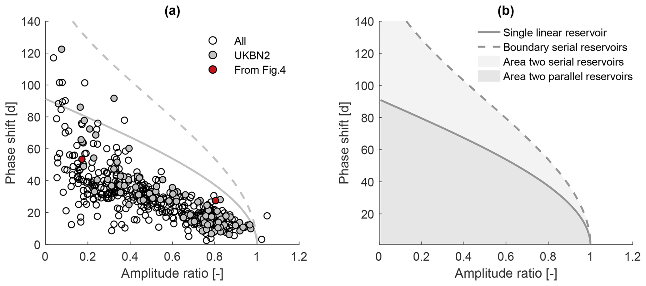
Figure 5(a) Amplitude ratio against phase shift for UK catchments. Grey dots indicate benchmark catchments, and red dots indicate the two catchments shown in Fig. 4. The grey solid line indicates a single linear reservoir, and the grey dashed line indicates the outer envelope for two reservoirs in parallel. Note that both axes are limited (two catchments are not shown). (b) Theoretical areas and limits for a single linear reservoir, two reservoirs in series, and two reservoirs in parallel.

Download

Figure 5a shows that most of the catchments fall below the solid grey line, which indicates the type of response that could be simulated by a single linear reservoir (see Fig. 5b). The area below the solid line can be simulated by two reservoirs in parallel. This would be the most parsimonious way to reproduce the observed behaviour if we decide to construct our model using linear reservoirs only. A few catchments plot above the solid line. For these catchments, the most parsimonious way to reproduce the pair of observed amplitude ratio and phase shift would therefore be two reservoirs in series. Very few catchments have an amplitude ratio larger than unity. While this could be caused by various errors in the data, it is likely due to erroneous catchment areas and/or the presence of inter-catchment groundwater flows or water transfers. If a catchment receives more net rainfall than the surface catchment area suggests (runoff ratio > 1), the amplitude in the output signal (streamflow) can be larger than the amplitude in the (erroneous) input signal.

4.3 Relationship between seasonal signatures and catchment attributes – UK

Figure 6 shows pairs of amplitude ratios and phase shifts, coloured according to different hydrological signatures and catchment attributes, respectively (explained in Table 1). Corresponding correlation coefficients can be found in Table 2. Figure 6a shows a clear pattern between the moisture index and the seasonal signatures. Generally, the less humid the catchments are, the lower the amplitude ratio is, and the larger the phase shift is. In other words, drier catchments attenuate the incoming forcing signal more strongly. This might partly be because we use potential evapotranspiration as our forcing. Lower actual evapotranspiration than potential evapotranspiration leads to a decreased input amplitude and thus to a higher amplitude ratio. Most of the very humid catchments plot close together, and the relationship between amplitude ratio and phase shift seems to be almost linear. Less humid catchments (note that in the UK none of the catchments are actually water-limited at the annual scale) show a larger spread, especially regarding the phase shift. Figure 6b shows a very similar pattern between the catchment wetness index and the seasonal signatures. Wetter catchments exhibit higher amplitude ratios and lower phase shifts, and vice versa. The catchment wetness index is strongly correlated with the moisture index (Spearman rank correlation of 0.94). Figure 6c shows a clear pattern between the baseflow index and the seasonal signatures. In contrast to the moisture index, where the stratification mostly follows the x axis (amplitude ratio), the stratification mostly follows the y axis (phase shift). Catchments with high BFIs exhibit low amplitude ratios and large phase shifts, and vice versa. Finally, in Fig. 6d we can see that catchments underlain by highly productive fractured aquifers exhibit (with a few exceptions) low amplitude ratios and large phase shifts.

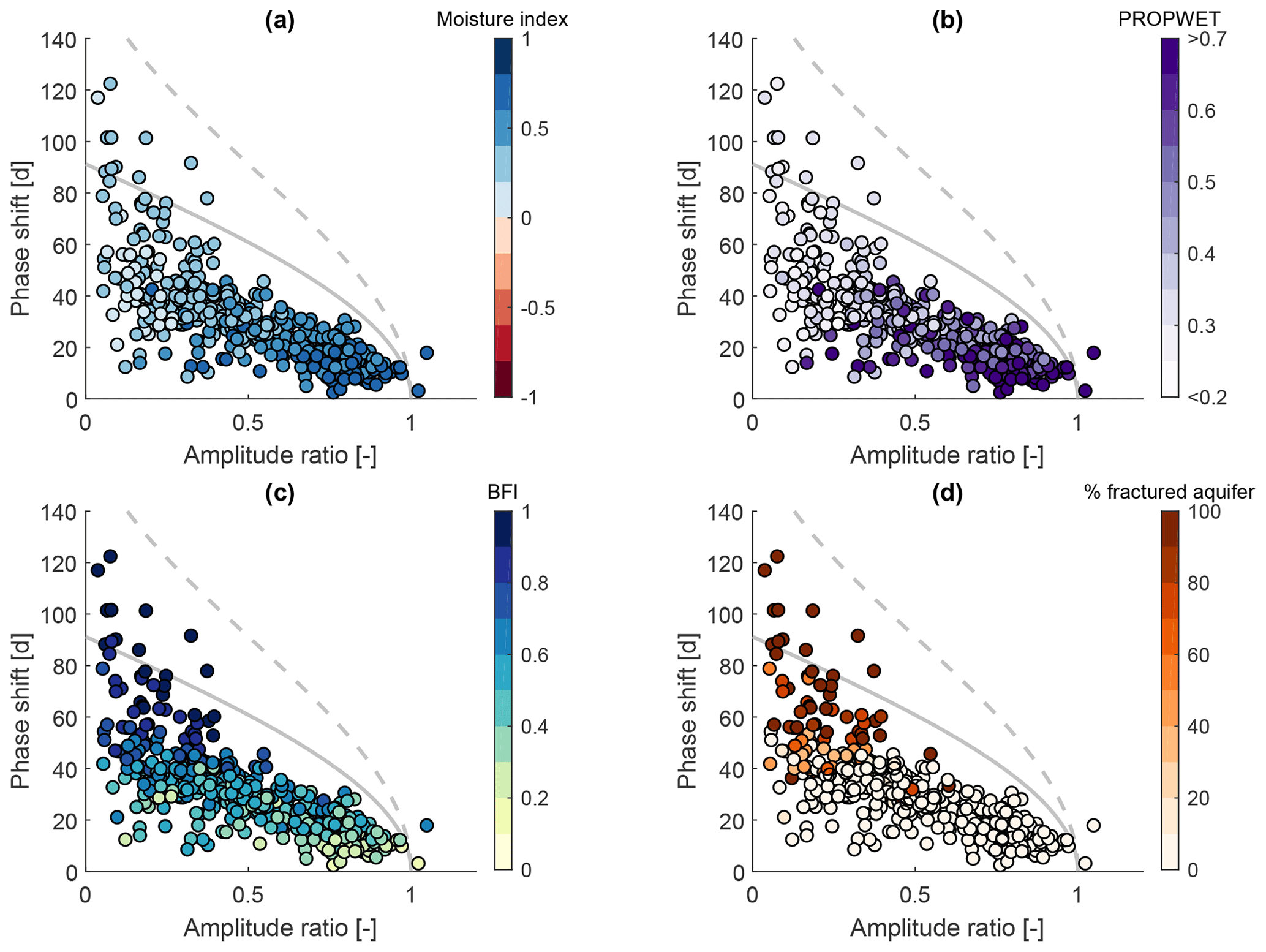
Figure 6Amplitude ratio against phase shift for UK catchments. The grey solid line indicates a single linear reservoir, and the grey dashed line indicates the outer envelope for two reservoirs in parallel. Colours indicate (a) the moisture index, (b) the catchment wetness index, (c) the baseflow index, and (d) the fraction of highly productive fractured aquifer. Note that both axes are limited (two catchments are not shown).

Download

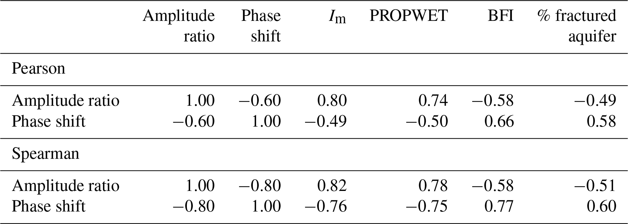
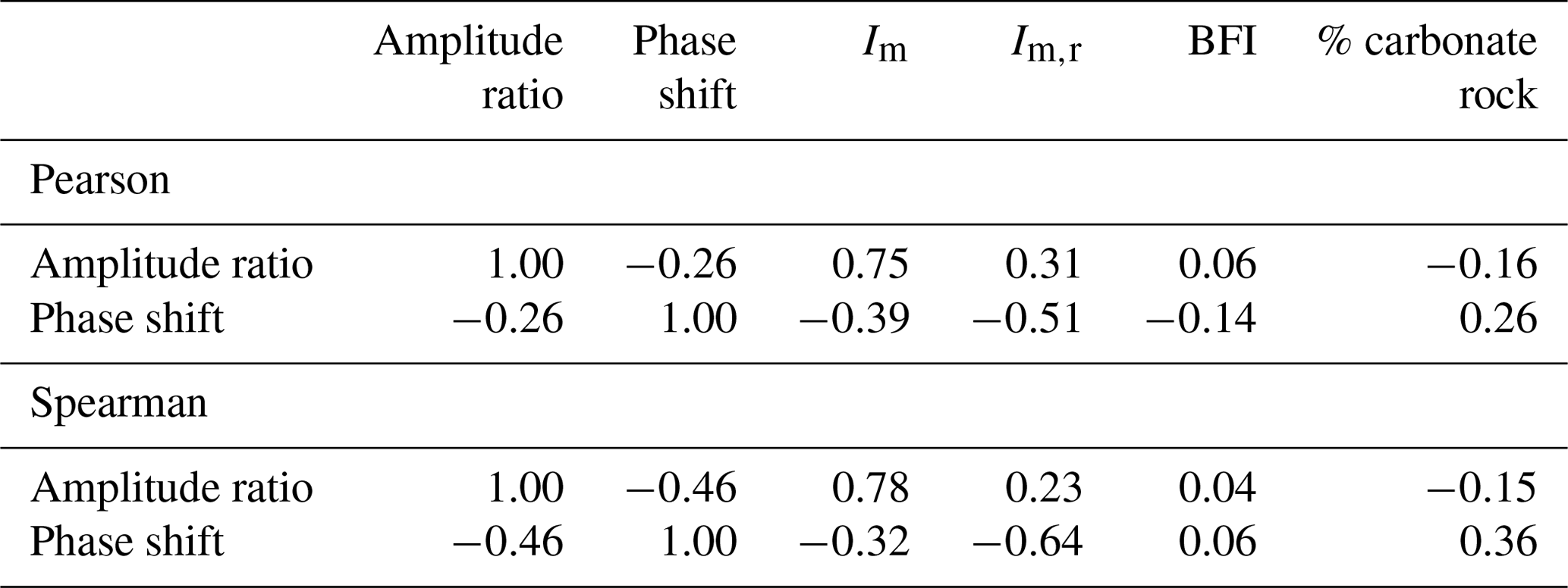
Table 2Pearson and Spearman correlation coefficients between seasonal signatures and catchment attributes for UK catchments.

Download Print Version | Download XLSX

4.4 Relationship between seasonal signatures and catchment attributes – US

Figure 7 shows pairs of amplitude ratios and phase shifts for the US, coloured according to different hydrological signatures and catchment attributes, respectively (explained in Table 1). Corresponding correlation coefficients can be found in Table 3. Catchments with a significant snow fraction (f_s>0.001) are removed, as snow presents another hydrological process which is not the focus of this study. Generally, snow adds another storage process, and this is reflected in large phase shifts observed in snowy catchments (see Sect. S2.3 for more information). The non-snowy catchments in the US show a similar trend to the catchments in the UK. Yet generally, the amplitude ratios are lower, and the phase shifts are larger compared to the UK (note that the y axes in Fig. 7 differ in their range from the y axes in Fig. 6). Humid catchments tend to have higher amplitude ratios and smaller phase shifts (Fig. 7a). Climate seasonality, indicated by the moisture index seasonality (see Fig. 7b), also influences the seasonal signatures. Catchments with a larger moisture index seasonality, i.e. a more variable monthly moisture index over the year, tend to have smaller phase shifts. The BFI (Fig. 7c) does not show such a clear pattern as for the UK catchments (Fig. 6c). Similarly, subsurface properties such as the fraction of carbonate sedimentary rock (Fig. 7d; and other attributes not shown here) only show a weak relationship with the seasonal signatures. Catchments with larger fractions of carbonate sedimentary rocks tend to have lower amplitude ratios and larger phase shifts. The overall pattern, however, is rather scattered. Contrary to the UK, some of the catchments in the US plot outside the area that can be modelled by either two reservoirs in series or in parallel, and some catchments have phase shifts larger than 182 d, the approximate limit for two reservoirs in series. These catchments are very arid and the low moisture seasonality index indicates that most of the precipitation in these catchments falls when potential evapotranspiration is highest, i.e. in summer.

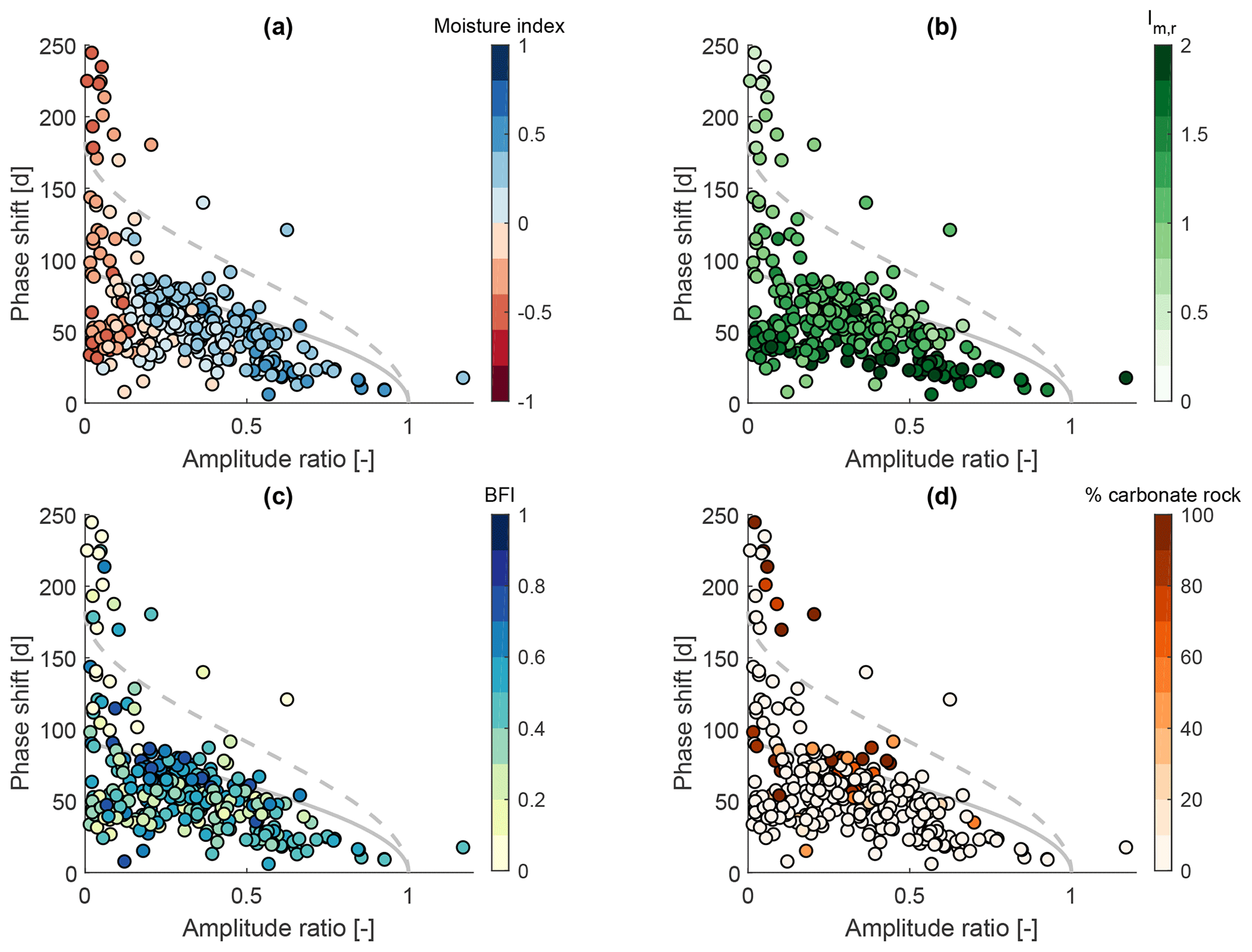
Figure 7Amplitude ratio against phase shift for CAMELS catchments. Catchments with a snow fraction (f_s>0.001) are removed from the analysis. The grey solid line indicates a single linear reservoir, and the grey dashed line indicates the outer envelope for two reservoirs in parallel. Colours indicate (a) the moisture index, (b) the moisture index seasonality, (c) the baseflow index, and (d) the fraction of carbonate sedimentary rock. Note that both axes are limited (12 catchments are not shown) and that the range of the phase shift axis is different from Fig. 6.

Download

Table 3Pearson and Spearman correlation coefficients between seasonal signatures and catchment attributes for CAMELS catchments.

Download Print Version | Download XLSX

4.5 Seasonal signatures as a diagnostic tool for evaluating hydrological models

In a similar fashion as for the observed catchment data, we now investigate the model runs using IHACRES and GR4J. Fig. 8 shows the resulting amplitude ratios and phase shifts for all model runs, that is for 20 000 parameter sets using data from a subset of 40 catchments in the UK. These plots show which combinations of seasonal signatures (and BFI) can be obtained with each model, given the forcing of 40 different catchments covering most of the hydro-climatic variability of the UK and given the parameter ranges chosen. They hence show the “signature space” of a model in the dimensions given by amplitude ratio and phase shift (and BFI).

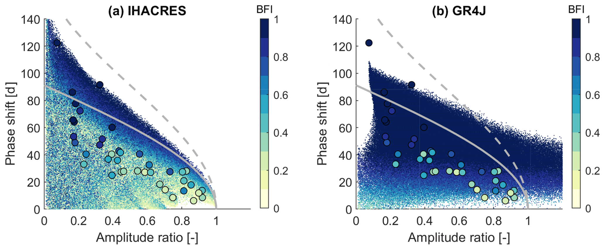
Figure 8Amplitude ratio against phase shift for 40 catchments in the UK using 20 000 parameter sets each for (a) IHACRES and (b) GR4J. The large dots show the observed signatures of the 40 catchments used for the modelling experiment. Colours indicate the BFI. Note that both axes are limited.

Download

IHACRES (Fig. 8a) shows a pattern that covers the area that can be modelled by two reservoirs in parallel and a large fraction of the area that can be modelled by two reservoirs in series (see Figs. 2 and 3). The BFI spans the whole range from 0 to 1. IHACRES can reproduce the observed amplitude ratios and phase shifts, although one catchment sits just at the boundary of the point cloud. GR4J (Fig. 8b) covers a different signature space. The phase shift never exceeds 105 d, the amplitude ratio often exceeds unity, and the BFI tends to be high. GR4J can reproduce most of the observed amplitude ratios and phase shifts, except for catchments with very large phase shifts. Furthermore, it struggles to simultaneously reproduce the observed phase shifts and BFIs. Both models sometimes yield phase shifts that are close to 1 year (not shown here), which are effectively negative phase shifts. A negative phase shift implies that the periodic component of Q leads the periodic component of P−E_p. This can happen if actual evapotranspiration E_a differs considerably from potential evapotranspiration E_p, and hence most of the input seasonality stems from P (and not E_p). This can be observed in a few catchments in the US (not shown here). It is only observed once in the UK (in a catchment with a man-made reservoir, not shown here), and therefore we do not investigate these model runs further.

Figure 9 shows distributions (“one-dimensional signatures spaces”) for three hydrological signatures for the 40 catchments investigated here. These plots tell us which signature values a model tends to produce (given a certain sampling scheme), the ranges of signatures a model can reproduce (given the parameter ranges chosen), and how (much) a signature varies with varying forcing.

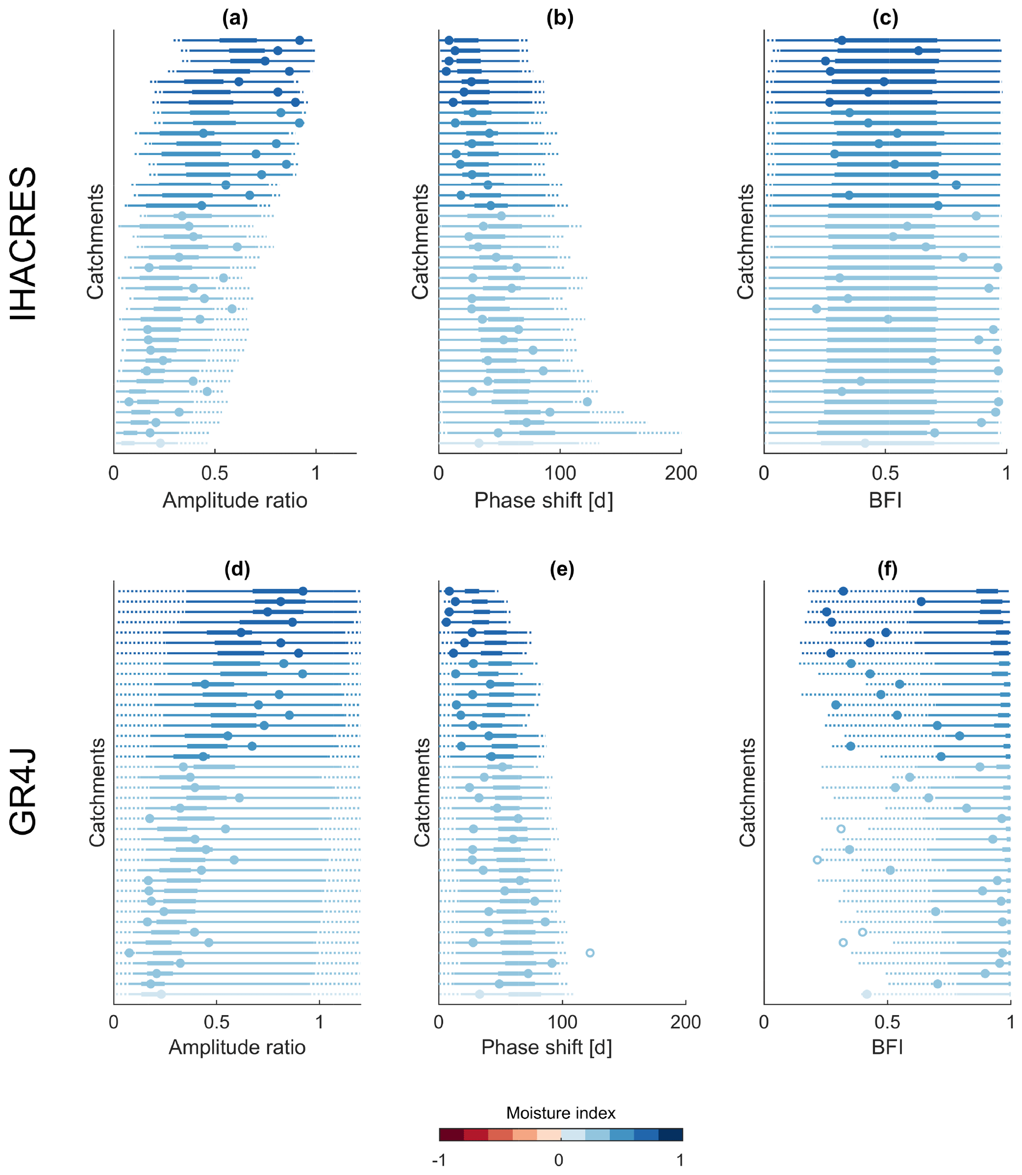
Figure 9Distributions of different hydrological signatures resulting from the modelling experiment. Each line stands for one of the 40 catchments, and the colours indicate the corresponding moisture index. The distributions of the modelled signatures are indicated by box-whisker-type plots. The thick line spans from the 25th to the 75th percentile. The thin line spans from the 1st (75th) to the 25th (99th) percentile. The dotted line indicates values below (above) the 1st (99th) percentile. The circles indicate the observed signature values, while filled circles indicate that the observed signature is inside the modelled signature space and vice versa. Panels (a), (b), and (c) show results for IHACRES. Panels (d), (e), and (f) show results for GR4J. Model runs with amplitude ratios lower than 0.01, amplitude ratios larger than 1.2, or phase shifts larger than 200 d have been removed.

Download

Figure 9 displays similar information as Fig. 8, yet it does not consider interactions between the three signatures. IHACRES can produce amplitude ratios from 0 to 1 and phase shifts up to 182 d (which is the limit for two reservoirs in series) and larger. GR4J can produce amplitude ratios that clearly exceed 1 and cannot model phase shifts larger than 105 d (given the parameter ranges chosen). For both models, more arid forcing leads to lower amplitude ratios and larger phase shifts, and vice versa. For the BFI (Fig. 9c and f) we can see that IHACRES covers the whole possible space (0 to 1) relatively evenly. GR4J tends to produce very high BFIs for almost every parameter set. BFIs smaller than 0.5 are possible with GR4J, but these are rather rare (or unlikely).

5.1 Representation of seasonal components by sine waves and limitations of the approach

A sine wave is a simple way of describing the seasonality of a signal. The results suggest that for most of the catchments investigated here, this approach is reasonable and efficient. Figure 4 shows that the average seasonal pattern is captured by the fitted sine waves. Differences between years cannot be captured by our approach, as we fit a single sine wave to describe the average seasonal behaviour. To robustly capture the average seasonal behaviour, we need relatively long time series. Comparing results from two different 10-year periods shows that the signatures are robust for the majority of catchments; i.e. their values do not differ substantially from one time period to the other (details are shown in Sect. S2.1.3).

The UK catchments and most of the US catchments exhibit a relatively strong unimodal (climate) seasonality (see e.g. Knoben et al., 2018). In other climates with a less distinct seasonal pattern, or with two seasons per year (Knoben et al., 2019b), our approach will not work. Semi-arid and arid catchments also tend to have a less smooth seasonal input, as water availability is more fragmented (Peters et al., 2003). Water-limited catchments can show a strong difference between potential evapotranspiration and actual evapotranspiration, which limits the applicability of our approach (we will discuss that later in more detail). We exclude catchments where precipitation is falling as snow. While snowy catchments are typically also strongly seasonal (Schaefli, 2016), this seasonality is mostly a climate phenomenon. It is rather related to temperature seasonality and not to the response of a catchment to periodic forcing.

5.2 A perceptual model of the seasonal response of catchments in the UK

The results, in particular Figs. 5 and 6 and Table 2, show clear patterns in the seasonal signatures. We can see that the seasonal response in the UK can be simulated by either two reservoirs in series or two reservoirs in parallel. This does not mean that there are no other configurations of more reservoirs leading to the same pairs of amplitude ratio and phase shift. Rather, two reservoirs in series and in parallel, respectively, are the most parsimonious reservoir configuration to reproduce the observed seasonal behaviour. Of course, two reservoirs in parallel and two reservoirs in series, respectively, might be seen as “special cases” of a soil reservoir followed by a fast and a slow reservoir, i.e. a three-reservoir arrangement. Furthermore, there might be concepts other than reservoirs which can explain the observed behaviour. Still, the observed patterns, both where the catchments plot for amplitude ratio vs. phase shift (Fig. 5) and how the catchment attributes relate to that (Fig. 6), suggest that the seasonal signatures are indeed a window into catchment functioning (Berghuijs et al., 2014) and thus have discriminatory power (McMillan et al., 2017; Addor et al., 2018).

Figure 6a and b shows how climate aridity and catchment wetness influence amplitude ratio and phase shift. The observation that more humid catchments respond more quickly to forcing (Fig. 6a and b) concurs with our understanding of these catchments. Wetter and therefore more saturated catchments partition the incoming water mostly into fast flow. The hydrograph closely resembles the forcing, which can also be seen in Fig. 4 for the responsive Ericht. The drier the catchments become, the more water is able to infiltrate, and subsurface properties become more important. This might explain why the spread becomes larger for less humid and hence less saturated catchments. In less humid catchments, actual evapotranspiration is more likely to deviate from potential evapotranspiration. This might be another reason for the greater attenuation in drier catchments, as the actual input (P−E_a) is lower than the theoretical one we compare to (P−E_p). In the UK the assumption that E_a=E_p seems reasonable (see Sect. S2.4 for further information). In more arid regions, such as parts of the US (see Sect. 5.3), this assumption is invalid.

The variability among UK catchments that cannot be explained by catchment wetness can mostly be explained by subsurface properties and the associated response time of a catchment. Catchments with high BFIs and thus large baseflow components show lower amplitude ratios and larger phase shifts, that is a more damped and lagged response (Peters et al., 2003). This can also be seen in Fig. 4 for the groundwater-dominated East Avon River. The relationship between BFI and the seasonal signatures (Fig. 6c) is not surprising, yet since the relationship is not unique, the seasonal signatures add another piece of information. In particular, the phase shift adds a timescale, which quantifies how long – on average – the seasonal input is delayed to become the seasonal output. While the phase shift is only a few days for the most responsive catchments, in the slowest catchments the seasonal signal is shifted up to 4 months. Since the BFI is rather a consequence of a catchment's hydrological behaviour (as are the seasonal signatures) than an attribute of a catchment, the BFI cannot be seen as a cause for the observed patterns in the seasonal signatures. It cannot be used, for example, as a predictor in ungauged catchments. A qualitative attribute that could theoretically be available in ungauged catchments, the fraction of highly productive fractured aquifer, reinforces the influence of the subsurface (Fig. 6d). Except for a few catchments, catchments underlain by such an aquifer exhibit very large phase shifts. In fact, all the catchments above the single reservoir line are underlain by highly productive aquifers. In these catchments, mostly underlain by Chalk, almost all the incoming water infiltrates into the aquifer, and the fast-flow component often is negligible. This might explain why they do not behave like reservoirs in parallel but rather like reservoirs in series, e.g. a soil reservoir (recharge) and a very slow groundwater reservoir. The few catchments which are underlain by highly productive aquifers, but do not exhibit large phase shifts, are typically overlain by rather impermeable drift, which stops water from infiltrating into the aquifer below.

Many models frequently used (and some of them developed) in the UK have a parallel flow structure, and catchments are usually conceptualised as having a fast and a slow component. While parametrisations and model structures vary between models, an overall parallel flow structure following a soil moisture module can be found in the probability distributed model (PDM; Moore, 2007), the TOPography-based hydrological MODEL (TOPMODEL) modelling concept (consisting of two fast flow responses; Beven and Kirkby, 1979), the IHACRES model (Croke and Jakeman, 2004), the GR4J model (Perrin et al., 2003), and many others. These or similar models have been applied to many catchments in the UK by various authors (e.g. Smith et al., 2019; Lane et al., 2019; Coxon et al., 2019). The seasonal signatures suggest that for most of the catchments, particularly if they are not underlain by a highly productive aquifer, a parallel model structure is a reasonable choice (at least for reproducing the response to seasonal forcing). For some groundwater-dominated catchments, however, the fast-flow component seems to be rather unimportant. Many of these catchments, typically catchments underlain by Chalk, could only be poorly modelled in national-scale modelling studies (Smith et al., 2019; Lane et al., 2019; Coxon et al., 2019). While this might partly be due to water balance problems (inter-catchment groundwater flows), it might also be due to an inadequate model structure or inadequate parameter ranges. The most parsimonious reservoir configuration for explaining the seasonal behaviour of these catchments (phase shifts > 91 d) would be two reservoirs in series, e.g. a soil or unsaturated zone reservoir transforming the incoming forcing into recharge and a (linear) groundwater reservoir. At least one of these reservoirs would need to be very slow to obtain such large phase shifts (cf. Fig. 2). For these groundwater-dominated catchments, a serial structure as it is also used in simple lumped groundwater models (e.g. Peters et al., 2003; Obergfell et al., 2019) seems to be a reasonable choice (at least for reproducing the response to seasonal forcing). As mentioned before, two reservoirs in parallel and two reservoirs in series, respectively, might be seen as “special cases” of a soil reservoir followed by a fast and a slow reservoir. For example, some of the catchments underlain by a highly productive aquifer fall in the area that can be simulated by two reservoirs in parallel (see Fig. 6d). Their large phase shifts and their proximity to the “single reservoir line” suggest, however, that the slow-flow component is of particular importance and that large time constants (>100 d) are required to model their behaviour.

In summary, the first control on the attenuation of the seasonal signal in the UK is the partitioning between fast flow and slow flow. More saturated catchments partition more rainfall into fast flow and hence lead to a higher amplitude ratio and to a smaller phase shift. The second control are catchment subsurface properties, which determine the available storage and how slowly water leaves the system. The slower the catchment responds, the larger the phase shift is, and the lower the amplitude ratio is. The Chalk catchments in the UK might be seen as an extreme case where almost all the water infiltrates, and hence the response time of a single slow reservoir (or perhaps two reservoirs in series) is the main control on the propagation of a periodic signal. On the other end of the spectrum, there are fully saturated, very responsive catchments mostly along the west coast of the UK, which behave almost like a single fast reservoir. Using conceptual reservoirs is only one way to interpret the seasonal signatures. It is useful as many hydrological models are built in that way. There might be, however, other possible ways of interpretation which we do not consider here.

5.3 A hydro-meteorologically more diverse set of catchments – the contiguous US

From Fig. 7 and Table 3 it can be seen that for CAMELS catchments (US) the climate indices explain most of the variability in the seasonal response. Again, more humid catchments tend to create more fast flow, and hence they have high amplitude ratios and small phase shifts. Catchments with a larger moisture index seasonality tend to have smaller phase shifts. In these catchments precipitation and potential evapotranspiration are mostly out of phase. Therefore, precipitation falls in more humid months, which might lead to a more flashy response. That means that both precipitation falling on wetter catchments and precipitation falling in wetter months will be less attenuated. The influence of catchment form is much less pronounced than in the climatically more homogeneous UK. Continental or global studies tend to identify climate as the dominant hydrological driving force (van Dijk, 2010; Beck et al., 2015), yet regional studies often show that other attributes such as geology are important (for baseflow, see e.g. Longobardi and Villani, 2008; Bloomfield et al., 2009). Our findings highlight anew that generalising from a global to a regional scale, or from a regional to a global scale, is not straightforward. Such scaling should ideally be done in a process-based way, or by analysing sub-climates, as the dominance of climate might mask the influence of other factors at large scales. We can also see that the attribute “fraction of highly productive fractured aquifers” (Fig. 6d), which is a hydrogeological classification available for the UK, shows a much clearer pattern than any soil or geology attributes in the US (see e.g. Fig. 7d which shows the fraction of carbonate sedimentary rock; the same is true if we use e.g. soil permeability for the UK). This might partly be due to the more heterogeneous US climate which masks the influence of subsurface properties to some degree. But it might also indicate that the soil or geology data used do not contain the hydrologically relevant soil or geology information. The hydrogeological classification based on expert judgement available for the UK, even though it is only categorical, might be more representative of the actual hydro(geo-)logical processes at the scale of interest. We therefore cannot conclude that in the US catchment form does not play a role. We can merely say that the catchment attributes used do not show clear patterns at the continental scale.

Some of the rather arid catchments in the US plot outside the area that can be modelled by two reservoirs in series or in parallel (Fig. 7). This either indicates that we would need another reservoir in series to model the observed phase shift (three reservoirs in series would result in a maximum phase shift of approximately 273 d), that (linear) reservoirs are not a good description of the hydrological processes, or that the proposed signatures are unreliable for these arid catchments. Since in water-limited catchments, actual evapotranspiration is typically much smaller than potential evapotranspiration, the input signal we use is very likely a poor proxy for the actual input signal. In very arid catchments ($I_{\mathrm{m}}<-\mathrm{0.5}$; dark red dots in Fig. 7a), particularly with the low moisture seasonality index (Fig. 7b), the results should therefore be interpreted with care. It is unclear to what extent these large phase shifts are the result of a poorly approximated input signal or actual catchment function. This compromises the consistency (McMillan et al., 2017) of the seasonal signatures and makes them most suitable for energy-limited catchments. A way to overcome this limitation would be the use of modelled or measured actual evapotranspiration as input data. As this would require another modelling step or additional data, we leave this for future work (see Sect. S2.4 for further information).

5.4 Can two common hydrological models reproduce the observed seasonal signatures?

The ensemble of IHACRES simulations covers the observed range of amplitude ratios and phase shifts, although one catchment sits just at the boundary of the point cloud (Figs. 8a and 9a–c). The BFI pattern also roughly resembles the observed pattern (Fig. 6c). Catchments with low BFIs tend to have high amplitude ratios and small phase shifts, and vice versa. To explain the signature space of IHACRES, it is useful to recall the structure of the model. IHACRES consists of a soil moisture deficit store, followed by two parallel linear reservoirs. It thus approximately features the two examples introduced in Sect. 2, namely two reservoirs in series or in parallel.

If one of the parallel reservoirs in IHACRES receives very little water (due to an extremely high or low fraction p going into the slow reservoir), the whole system acts like two reservoirs in series. The only difference is that the first reservoir is not a single linear reservoir. It is a non-linear deficit store and thus different from the idealised linear reservoir. This might explain why the upper boundary looks similar to the grey dashed line indicating two linear reservoirs in series, yet it does not look exactly the same. We did explore how non-linear reservoirs behave in terms of amplitude ratio and phase shift, and they seem to behave similar to linear reservoirs (see Sect. S1.4). Another reason for IHACRES not covering the whole area might be the parameter ranges (see Sect. S3 for details). The parameter ranges used are intended to be wide, yet especially the fast reservoir (in order to be indeed fast) is limited to 10 d, which limits the theoretical space to be smaller than shown in Fig. 2.

If the soil moisture reservoir transmits water relatively quickly without much attenuation, the whole system acts like two reservoirs in parallel. In summary, IHACRES is very similar to the idealised arrangement we introduced in Sect. 2, and this can be seen in the model output. It is therefore likely that IHACRES is capable of reproducing the observed seasonal signatures for catchments in the UK (Fig. 6) and for most of the catchments in the US (Fig. 7). Whether IHACRES can reproduce the seasonal signatures, other hydrological signatures and achieve satisfactory statistical performance metrics simultaneously is to be explored and beyond the scope of this paper.

The ensemble of GR4J simulations covers most of the amplitude ratios and phase shifts observed in the UK (Figs. 8b and 9d–f). Many of the model runs lead to amplitude ratios higher than unity, which is caused by the groundwater exchange parameter, which allows the model to import water in addition to incoming P. While this is possible (and can in fact be observed; e.g. in Fig. 6c the blue dot outside the grey boundaries is a catchment with water transfer from a neighbouring catchment), it is observed very rarely in the catchments investigated. Furthermore, a non-zero groundwater exchange parameter should ideally be associated with actual water inputs or outputs (e.g. inter-catchment groundwater flows), and these inputs or outputs are usually unknown. It is worth noting that many model runs that lead to signature values at the boundaries of the signature space (e.g. low BFIs or large phase shifts) are associated with large (positive or negative) values for the groundwater exchange parameter (not shown here). This might further reduce the “realistic” signature space, as, for example, obtaining a low amplitude ratio by removing water might be seen as “the right answer for the wrong reason”. No model run leads to a phase shift larger than about 105 d. GR4J also has a soil moisture store followed by two parallel routing stores; i.e. the overall model structure is similar to IHACRES. The stores are, however, not linear reservoirs. In addition to that, GR4J has fixed internal parameter values, such as the fraction of water going through the slow routing store, which is set to 0.9. This might explain why the BFI tends to be very high, as it can be seen from Fig. 9f. Despite the tendency towards large BFIs, GR4J cannot produce phase shifts larger than about 105 d given the parameter ranges used here. This might be due to a range of the flow delay parameter which is too narrow (maximum 15 d). So, to model both the phase shift and the BFI correctly, we might require a more flexible splitting between fast and slow routing and a means to produce larger phase shifts (e.g. via a wider range for the flow delay parameter).

Figure 9 also shows how the seasonal signatures (and the BFI) vary with different inputs (forcing). For both models, more humid catchments lead to higher amplitude ratios and smaller phase shifts, and vice versa. This trend, not necessarily the values themselves, agrees with the observed behaviour shown in Figs. 6a and 7a.

This analysis is necessarily incomplete for (at least) two reasons. First, we only looked at 40 catchments in the UK to limit the computational demand. Therefore, the conclusions are not necessarily transferable to catchments outside the UK. More arid catchments (e.g. in the US) might show a different behaviour (e.g. the catchments showing phase shifts larger than 182 d; see Fig. 7). Second, the sampling scheme (Latin hypercube sampling) explores only a subspace of the actual parameter values (both because of the parameter ranges and because of the finite amount of parameter sets). We also made an a priori decision of how to sample by choosing Latin hypercube sampling in the first place. This is inevitably subjective, and other sampling schemes might lead to different results. This might especially affect the distributions of the modelled signatures shown in Fig. 9. Wider parameter ranges might change the ranges of the resulting signature spaces. As we use rather wide ranges based on recent literature (see Sect. S3 for details), our results should (at least) be representative of current modelling practice. This kind of analysis and the seasonal signatures can therefore help to select (or not select) models a priori, without calibrating them to streamflow data (cf. Vogel and Sankarasubramanian, 2003). This might be particular helpful for large sample studies where often a certain model structure is chosen a priori, even if it might be inadequate for the catchment sample investigated (Addor and Melsen, 2019).