the Creative Commons Attribution 4.0 License.
the Creative Commons Attribution 4.0 License.
 | 17 Feb 2020
Multimodel simulation of vertical gas transfer in a temperate lake
Sofya Guseva
Tobias Bleninger
Klaus Jöhnk
Bruna Arcie Polli
Zeli Tan
Wim Thiery
Qianlai Zhuang
James Anthony Rusak
Huaxia Yao
Andreas Lorke
Victor Stepanenko
In recent decades, several lake models of varying complexity have been developed and incorporated into numerical weather prediction systems and climate models. To foster enhanced forecasting ability and verification, improvement of these lake models remains essential. This especially applies to the limited simulation capabilities of biogeochemical processes in lakes and greenhouse gas exchanges with the atmosphere. Here we present multi-model simulations of physical variables and dissolved gas dynamics in a temperate lake (Harp Lake, Canada). The five models (ALBM, FLake, LAKE, LAKEoneD, MTCR-1) considered within this most recent round of the Lake Model Intercomparison Project (LakeMIP) all captured the seasonal temperature variability well. In contrast, none of the models is able to reproduce the exact dates of ice cover and ice off, leading to considerable errors in the simulation of eddy diffusivity around those dates. We then conducted an additional modeling experiment with a diffusing passive tracer to isolate the effect of the eddy diffusivity on gas concentration. Remarkably, sophisticated k−ε models do not demonstrate a significant difference in the vertical diffusion of a passive tracer compared to models with much simpler turbulence closures. All the models simulate less intensive spring overturn compared to autumn. Reduced mixing in the models consequently leads to the accumulation of the passive tracer distribution in the water column. The lake models with a comprehensive biogeochemical module, such as the ALBM and LAKE, predict dissolved oxygen dynamics adequate to the observed data. However, for the surface carbon dioxide concentration the correlation between modeled (ALBM, LAKE) and observed data is weak (∼0.3). Overall our results indicate the need to improve the representation of physical and biogeochemical processes in lake models, thereby contributing to enhanced weather prediction and climate projection capabilities.
- Article
(3819 KB) -
Supplement
(4278 KB) - BibTeX
- EndNote


The past 2 decades have seen a renewed interest in lake modeling. Due to the ever-increasing spatial resolution in numerical weather prediction systems and climate models, many lakes became resolvable on the model grid. Lakes are responsible for changing local atmospheric conditions by modifying turbulent fluxes of heat, moisture and momentum relative to adjacent land (Forbes and Meritt, 1984; Mahrt, 2000; Long et al., 2007; Thiery et al., 2015). This effect can be substantial over regions where the total coverage of inland water bodies is high, e.g., in Finland or Sweden (≈10 %, 9 % lakes of the total area, respectively (Lehner and Döll, 2004)), or where large lakes dominate (Docquier et al., 2016; Thiery et al., 2015, 2016, 2017). Additionally, lakes are increasingly recognized as a considerable source of greenhouse gases, such as carbon dioxide (CO2) and methane (CH4), to the atmosphere (Tranvik et al., 2009; Bastviken et al., 2011; Raymond et al., 2013; Tan and Zhuang, 2015; Wik et al., 2016).
With the development of multiple lake models of varying complexity, it becomes necessary to compare them and examine their merits and drawbacks in the context of atmospheric and limnological applications. The scientific community has addressed this need through the Lake Model Intercomparison Project (LakeMIP) launched in 2008 (http://netfam.fmi.fi/Lake08/, last access: 16 February 2020). Since then, a methodology for lake model comparison has been developed (Stepanenko et al., 2010), and lake model intercomparison experiments have been conducted for a range of limnological and climatic conditions. In each experiment, input parameters were unified as much as possible, including identical meteorological forcing, optical properties of water, ice, and snow, initial temperature profiles, and lake depth and/or morphometry. This allowed for a detailed inter-model comparison in respect of limnophysical process representation.
Previous LakeMIP studies primarily investigated the ability of the lake models to simulate the thermal regime of the water bodies that cover a wide range of size, depth and mixing regimes at different latitudes. In particular, the major effort has been spent on the simulation of the evolution of the vertical temperature profile along with the surface temperature and energy fluxes to the atmosphere. At the same time, biogeochemical processes were not considered in the model intercomparison studies.
LakeMIP simulations have been performed using seven 1-D lake models: (1) CLM4-LISSS (Hostetler and Bartlein, 1990; Subin et al., 2012), (2) FLake (Mironov, 2003), (3) Hostetler model (Hostetler et al., 1993), (4) LAKE (Stepanenko et al., 2011, 2016), (5) LAKEoneD (Jöhnk and Umlauf, 2001; Jöhnk et al., 2008), (6) MINLAKE96/2012 (Fang and Stefan, 1996), and (7) SimStrat (Goudsmit et al., 2002). They targeted deep lakes, monomictic Lake Geneva (Switzerland/France), dimictic Lake Michigan (USA), and meromictic equatorial Lake Kivu (central Africa), and for shallow lakes, Lake Sparkling (USA), Großer Kossenblatter See (Germany), and Lake Valkea-Kotinen (Finland). The lake models in general simulated reasonable seasonal variability of temperature and thermocline characteristics (Perroud et al., 2009; Stepanenko et al., 2010). However, the simulated and observed evolutions of the mixed-layer thickness and the bottom temperature tend to disagree. The k−ε models (SimStrat, LAKE, LAKEoneD) demonstrate intensive mixing of the lakes during summer, emphasizing their applicability especially to shallow lakes (Stepanenko et al., 2010, 2014). Nevertheless, these types of lake models can also be appropriate for studying physical processes in deep lakes (Thiery et al., 2014a). Furthermore, lake models using the Henderson-Sellers parameterization of vertical mixing (e.g., CLM4-LISSS, Hostetler lake model, Henderson-Sellers, 1985) represent the thermodynamic state of a water body adequately, but can underestimate mixolimnion temperatures (Thiery et al., 2014a). The FLake model has demonstrated less satisfactory agreement with observations in terms of summer stratification in previous studies, yet simulates surface temperatures well.
This paper presents a logical continuation of LakeMIP by advancing intercomparisons to the study of biogeochemical processes in lakes. It primarily focuses on the simulation of key physical factors affecting the vertical transport of greenhouse gases, such as thermal stratification, vertical diffusion of gases, and ice cover. The ice cover is of special interest for greenhouse gas dynamics, as it can cause the depletion of oxygen, which favors CH4 accumulation until spring ice breakup (Phelps et al., 1998; Karlsson et al., 2013; Jammet et al., 2015).
Our study aims at identifying the major merits and shortcomings of different lake model formulations, as well as uncertainties in simulating the limnophysical controls on greenhouse gas distribution and emissions to the atmosphere. Simulations were run for Harp Lake, a lake in Ontario, Canada, with long-term high-frequency monitoring data for meteorology, water temperature, CO2 and O2. Five lake models were used in this study to simulate thermal dynamics and turbulent diffusivity in the lake: (1) Arctic Lake Biogeochemistry Model, ALBM (Tan et al., 2015, 2017, 2018; Tan and Zhuang, 2015), (2) FLake (Mironov, 2003), (3) LAKE (Stepanenko et al., 2011, 2016), (4) LAKEoneD (Jöhnk and Umlauf, 2001; Jöhnk et al., 2008), and (5) Modelagem do Transporte de Calor no Reservatório, MTCR-1 (Polli and Bleninger, 2015, 2018). The ALBM and LAKE models include comprehensive biogeochemical modules for calculation of dissolved gas concentrations, which were then tested in their ability to reproduce CO2 and oxygen O2 dynamics. The study is structured as follows: Sect. 2 includes the description of the study site, observational data, lake models, and experimental setup. Section 3 is devoted to the simulation of the lake's thermal regime, i.e., the temperature patterns and eddy diffusivity (ED). To assess the pure effect of the ED on the gas distribution and dynamics in the lake, additional experiments have been conducted, where the fate of passive tracers emitted from the bottom of the lake was analyzed. In a final section, the ALBM and LAKE models are compared in terms of the CO2 and O2 concentration in Harp Lake.
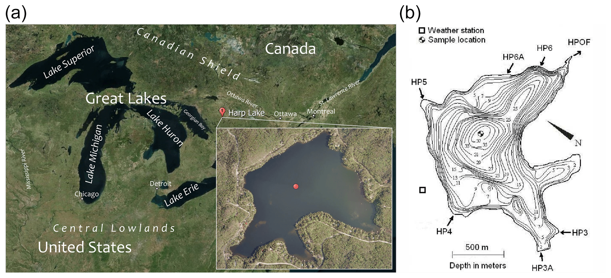
Figure 1The location and morphometry of Harp Lake (HP3 to HP6A are the six inflows; HPOF is the lake outflow). Red circle indicates the position of the high-frequency monitoring buoy (45∘22′44.88′′ N, 79∘8′7.77′′ W). (a) Map data copyright 2017 by © Google, Maxar Technologies; (b) reprinted from Yao et al. (2014), copyright 2014 by Hydrol. Process.
2.1 Study site and data
2.1.1 Study area
The object of the current study is Harp Lake (45∘22′ N , 79∘07′ W, 327 m a.s.l. – above sea level), a dimictic temperate lake located in southern-central Ontario, Canada. The lake and its surrounding forested catchment are representative of the southern Canadian Shield landscape (Cox, 1978; Dillon et al., 1987) (Fig. 1). It has a 0.71 km2 surface area, a volume of 0.0095 km3, a maximum depth of 37.5 m and a mean depth of 13.32 m. The lake is oligotrophic, characterized by average total phosphorus and chlorophyll-a concentrations of 6.7 and 3.5 µg L−1 (Molot and Dillon, 1991). The water is slightly acidic (pH 6.3) (Dillon et al., 1987). Harp Lake has six inflows and one outflow, with a long-time average discharge of 0.067 m3 s−1 for the inflows and 0.091 m3 s−1 for the outflow. The difference is due to small ungauged inflows and overland flow. Its average residence time is 3.1 years. Due to this relatively long residence time, the effect of the inflows on temperature can be neglected. The lake has only small water level fluctuations (maximum ∼ 0.2 m).
2.1.2 Observational data
The lake has been monitored by the Dorset Environmental Science Centre (DESC) for more than 40 years, thus providing a comprehensive database supporting the model experiments. The high-frequency and continuous observations used in this study have been collected during 5 years (14 July 2010–19 October 2015) with 10 min resolution on a monitoring buoy in the lake center (Fig. 1). The meteorological variables collected are air temperature, humidity at a height of 1.75 m above the water surface, wind speed at 1.75 m, and downwelling shortwave and longwave radiation. Pressure and precipitation are available from a land-based meteorological station 500 m away from the western lake shore. The high-frequency dataset further includes a vertical temperature profile (up to a depth of 27.1 m prior to the summer of 2012 and to a depth of 9.85 m thereafter, aggregated to a time step of 1 h), O2 concentrations (at two depths: 1, 18 m, aggregated to a time step – 1 h) and CO2 concentration (at a depth of 0.39 m, for the period 12 March 2012–19 October 2015, aggregated to a time step of 1 h). In addition, traditional temperature and O2 profiles were collected to a depth of 35 m, except during the wintertime period, at a time step of approximately 2 weeks, and Secchi depth was also measured fortnightly or monthly during these 5 years (for more details, see Tables S6 and S7).
The meteorological conditions of the region during the period under study are typical for continental climate of mid-latitudes (Table 1). This region is subject to the influence of the Azores High during summer and is located in between the Icelandic Low and the Canadian High forming in the central part of the continent during winter. Cold arctic air usually invades this area during winter, leading to the formation of stable freezing weather. However, it should be considered that winters are usually characterized by several abrupt rises in air temperature above 0 ∘C (see Fig. S1 in the Supplement). This phenomenon causes the 2012 winter to rank as the warmest winter during the 5 measurement years. Average annual wind speed is relatively low (≈2 m s−1), likely caused by wind-shading effects imposed by the surrounding forest. Predominant wind directions are WSW (230–280∘) and SE (130∘).
Table 1Hydrometeorological conditions during the period 14 July 2010–19 October 2015.
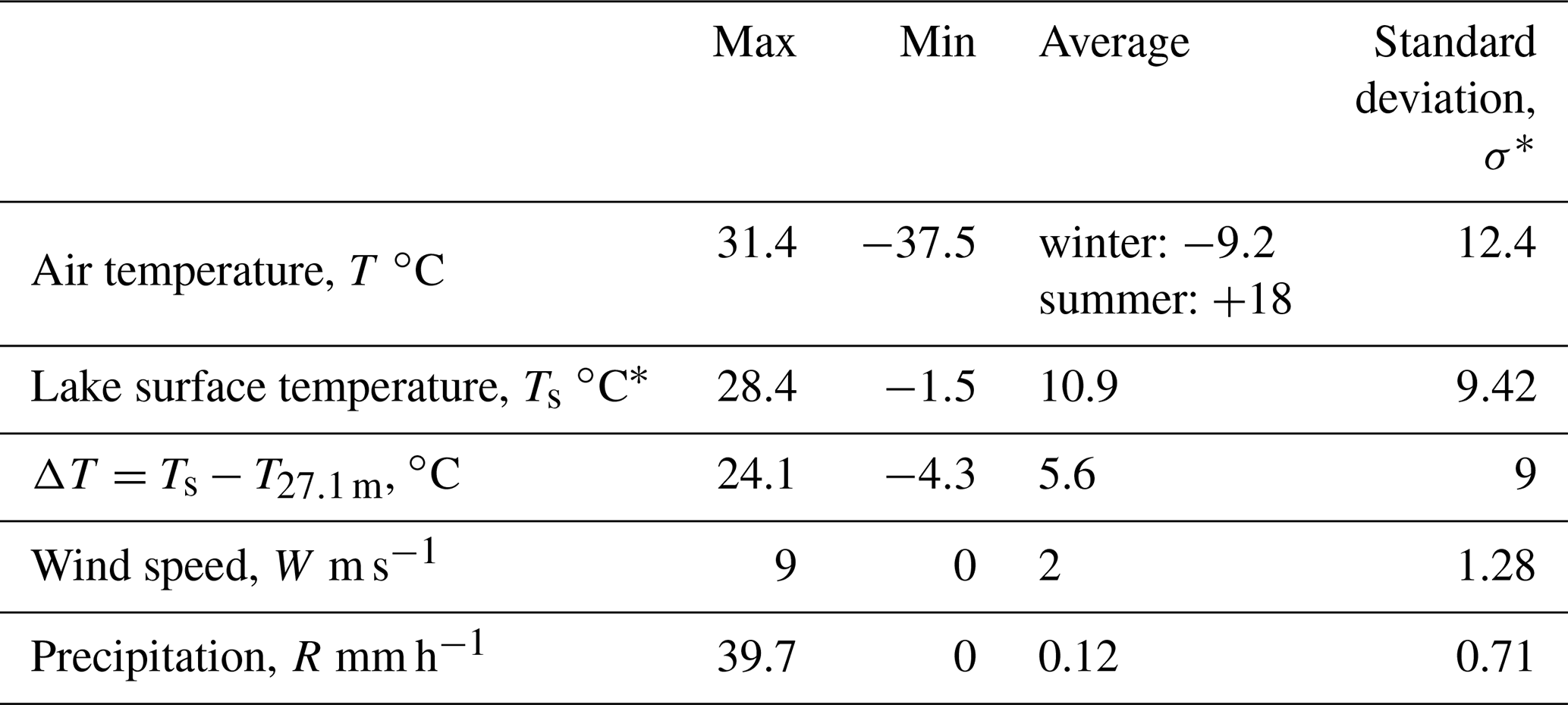
* Water temperature measured at 0.1 m depth.
2.2 Lake models
In this study, a suite of 1-D lake models was applied to Harp Lake. Two classes of finite difference models can be identified based on different approaches of calculating the vertical ED: Henderson-Sellers-based models (Henderson-Sellers, 1985; Hostetler and Bartlein, 1990), which are computationally inexpensive, and the more sophisticated models based on the k−ε turbulence closure scheme. The Henderson-Sellers approach computes the ED coefficient as a function of the Richardson number and considers wind-driven turbulence during stable or neutral stratification. A separate procedure is considered for convective mixing and assumes instantaneous mixing of unstably stratified depth layers. The k−ε formulation involves prognostic equations for turbulent kinetic energy and its dissipation. Both wind-induced and convective turbulence are taken into account in this approach. Within the first class there are the recently developed models ALBM and MTCR-1, while k−ε models include LAKE and LAKEoneD.
The FLake model stands aside from the other 1-D models due to the two-layer bulk structure which employs the concept of self-similarity to estimate the temperature profile in the mixed layer and thermocline, respectively (Mironov, 2008). In the mixed layer the temperature is assumed to be constant, whereas below it is parameterized as a function of non-dimensional depth. ED is not explicitly specified in this model. Of all models, FLake has the lowest computational cost (Thiery et al., 2014a).
Ice formation is one of the main controlling factors for the dissolved gas dynamics in a lake during winter. Models like LAKEoneD and MTCR-1 involve a simple ice parameterization, in which ice cover is governed only by air temperature and lake temperature is not considered (Ashton, 1980, 2011). In the FLake model, the temperature profile within the ice cover is parameterized via a time-varying shape function with a linear asymptotic. The ALBM incorporates a more comprehensive ice parameterization developed by Fang and Stefan (1994), taking into account the physical processes of freezing of the surface water, radiation and heat penetration through ice and snow. The LAKE model takes into account the same physical processes and uses a multilayer ice parameterization (Stepanenko and Lykossov, 2005; Stepanenko et al., 2011) based on an unsteady heat transfer equation. Light extinction in all models follows the Beer–Lambert law with a constant light attenuation coefficient.
The ALBM and LAKE incorporate the most comprehensive biogeochemical modules, including the sources, sinks and transport of CO2, O2, and CH4 (and nitrogen in the ALBM) (see Table S1 in the Supplement). LAKEoneD model calculates O2 concentration only. Parameters and characteristics of all models are summarized in Table 2. All the models use finite-difference numerical schemes along vertical coordinates, except for FLake, which is based on the two-layer representation of the lake temperature profile (see above). The vertical grid of these models is fixed in time, while the number of numerical layers varies from 51 to 105 between models. The time step varies within the range of 20–3600 s between the models. The ALBM uses a fourth-order adaptive Runge–Kutta–Fehlberg solver and a variable time step. If there are abrupt changes in boundary conditions (such as air temperature, solar radiation and wind), the time step in this model will be reduced to avoid numerical instability.
(Fang and Stefan, 1994)(Ashton, 1980, 2011)(Stepanenko and Lykossov, 2005)(Ashton, 1980, 2011)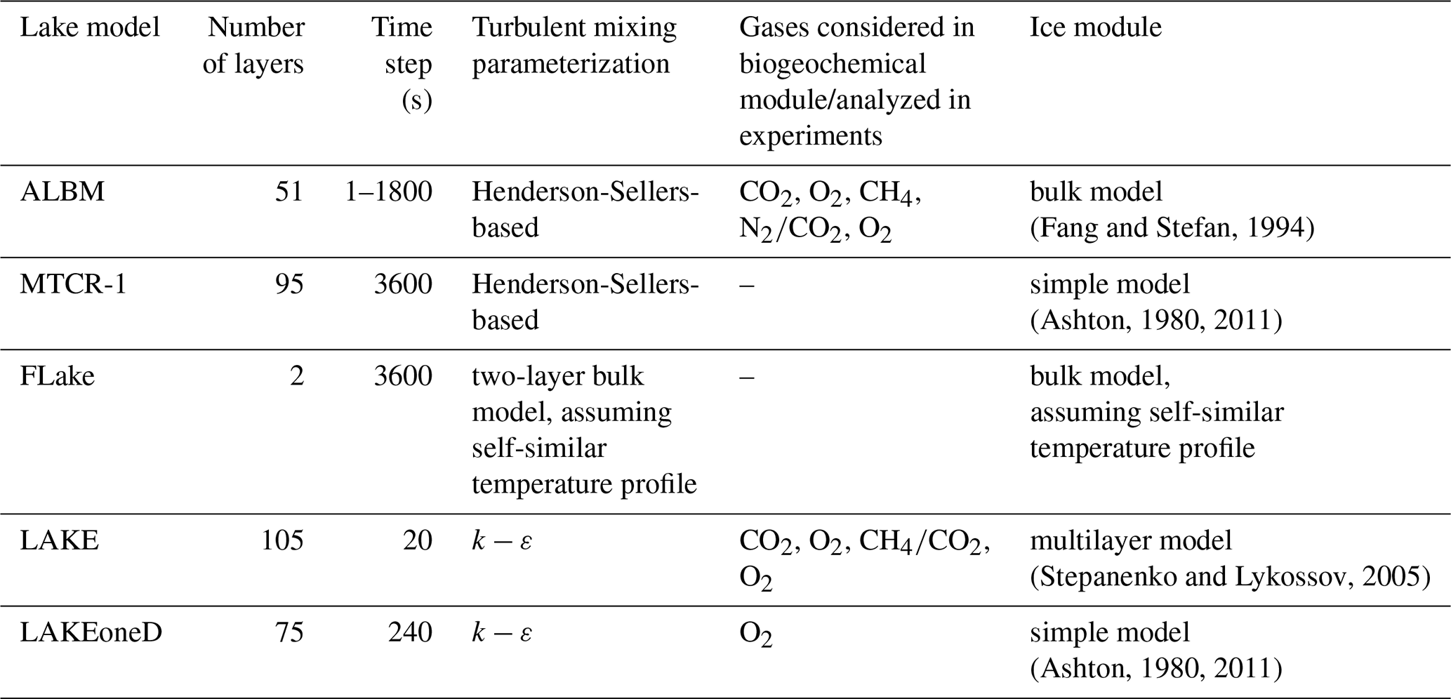
2.3 Experimental setup
In this study, a set of numerical experiments was conducted to compare model simulation outputs assuming different morphometries, light extinction coefficients, and for the biogeochemical model parts initial CO2 concentrations (Table 3):
-
a reference simulation in which the depth is set to a maximum value (37.5 m), light attenuation coefficient is set to a mean measured value (μ=0.4 m−1) and the morphometry is not taken into account (dependence of horizontal cross-section area on depth (hypsometric curve) is not included) (RefSim);
-
model simulations testing the sensitivity of models to variations in
-
lake depth, setting it to mean value have=13.32 m (LDSim),
-
the light attenuation coefficient, prescribing μmin=0.28 m−1 and μmax=0.68 m−1, which are minimal and maximal values measured, respectively (ExtMinSim, ExtMaxSim),
-
-
a model simulation testing the effect of the vertical diffusion on the distribution of the passive tracer (PassTrSim), and
-
a model simulation with biogeochemical modules activated including the calculation of the O2 and CO2 concentration (GasSim). Measured mean CO2 concentration and O2 observations are used as initial profiles. The time step of model output in all experiments is 1 h.
Table 3Parameters of numerical experiments of LakeMIP-Harp.
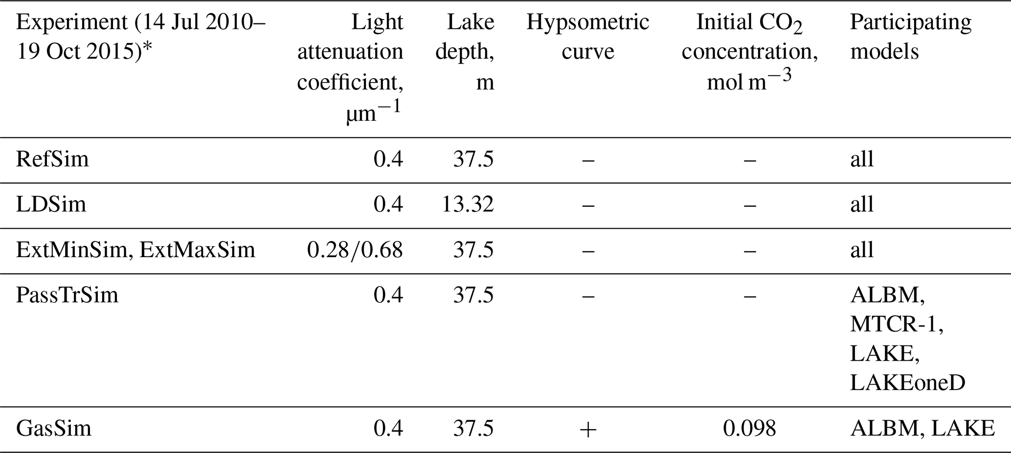
* For more details, see the simulation protocol in SI. Some of the experiments are not included in our study.
The concept of the self-similarity in the FLake model (Sect. 2.2) includes the “shape factor” coefficient Cθ, which determines the vertical temperature profile below the mixed layer. Evolution of this parameter is controlled by a relaxation timescale trc (Mironov, 2008). This timescale includes the dimensionless relaxation constant Crc with a default value of 0.003 in the model. This constant is a calibration parameter which is generally individual for each lake (Shatwell et al., 2016; Kirillin et al., 2017). We tested the sensitivity of the model to the variation of Crc using values 0.03, 0.3, 0.5, 1, 2, 3, and 30 and achieved the best agreement with the measured temperature profile using Crc=0.3 (for details, see Sect. 3.1). In the following sections, this Crc setting is used in RefSim and other experiments with the FLake model.
The meteorological forcing is identical for all models and experiments. This, however, does not imply that heat fluxes to the atmosphere are the same in models, as models use different surface flux schemes. Some of the models do not include bathymetry (e.g., FLake); thus, for a more consistent comparison, in the RefSim experiment all models are integrated assuming homogeneous depth. In the GasSim experiment, lake morphometry is considered because the lake's carbon budget cannot be accurately calculated without including sediment oxygen demand along a sloping bottom.
The effect of the tributaries is neglected due to the large residence time of Harp Lake. Likewise, water-level variations are not considered in the models given the small temporal fluctuations.
The choice of the lake depth in the 1-D model without bathymetry may be crucial for the modeling results, not only for the temperature regime (Balsamo et al., 2010), but also for the gas dynamics. The gas dynamics is affected by lake depth as the latter controls the amount of bottom-originated gas to be biochemically transformed in the water column (e.g., oxidation of CH4). Thus, it is important to examine the sensitivity of models to this parameter. In all experiments except LDSim, the maximal depth is used to compare the output with all available measurements. To test the effect of the chosen depth on model performance, the depth is set to mean depth (13.32 m) in the LDSim experiment; as such, the modeled lake volume is equal to the real lake volume.
The light attenuation coefficient is an important parameter, regulating the thermal regime of a lake (Heiskanen et al., 2015) and biogeochemical processes including photosynthesis. Secchi depth measurements during the 5-year study period on Harp Lake are irregular but enable calculation of mean, maximum and minimum light attenuation coefficients using the Poole and Atkins formula (Poole and Atkins, 1929).
The motivation for conducting experiments with perturbed input parameters (depth and light attenuation coefficient) and initial conditions (dissolved gases) is that these properties, especially the light attenuation coefficient, become considerably uncertain in global applications. While a first global lake depth database recently became available (Choulga et al., 2014; Kourzeneva, 2010), such a dataset currently does not exist for water transparency.
To understand the role of the ED coefficient in gas distribution and dynamics, an additional experiment solving the pure vertical diffusive transport equation for a passive tracer governed by eddy diffusivities resulting from different lake models was conducted. Details on this experiment are presented in Sect. 3.3.
Harp Lake is a deep lake suitable for studying the transport of O2 and CO2 as well as their biogeochemical transformations due to long-term regular measurements of these gases. In this respect, the additional numerical experiment (GasSim) was conducted with the ALBM and LAKE, the lake models with the most sophisticated biogeochemical modules. To harmonize the experimental setup, the contribution of CO2 and O2 fluxes through a sloping bottom to the lake carbon budget was switched on in the LAKE model. It should be noted that the ALBM includes a CO2 sink/source due to outlets and inlets, whereas LAKE does not take this effect into account. In the ALBM, a set of biogeochemical parameters was calibrated, specifically, maximum chlorophyll-specific photosynthetic rate, maximum metabolic loss potential, aquatic dissolved organic matter (DOM) microbial degradation rate, terrestrial DOM microbial degradation rate, and groundwater dissolved organic carbon (DOC) concentration (Tan et al., 2017). No parameter calibration was performed for the LAKE model (a complete set of default values of model parameters is given in Stepanenko et al., 2016).
The model skill scores used in this study are listed in Table 4.
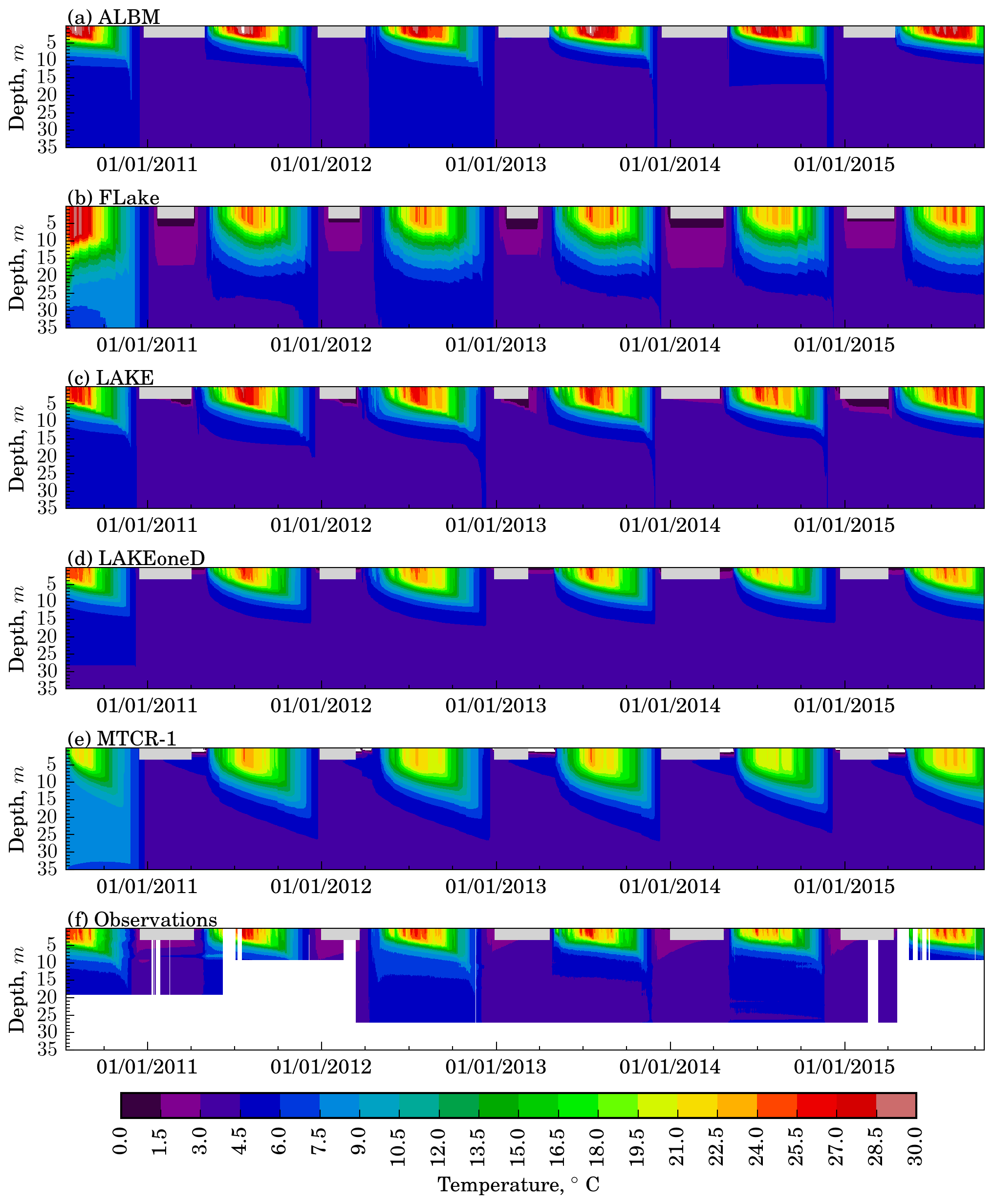
Figure 2Time–depth pattern of temperature in Harp Lake (14 July 2010–19 October 2015), RefSim and observed data. The grey boxes represent the duration of the ice-cover period, and the white patterns denote the absence of data.

3.1 Temperature and ice
All the lake models simulate seasonal water temperature dynamics adequately (Fig. 2): the epilimnion is warming throughout the first half of summer, accompanied by thermocline deepening, eventually leading to overturn in autumn. During winter, the lake temperature is at the freezing point immediately below the ice cover, causing stable stratification. During spring, the lake starts to mix due to the penetration of shortwave radiation. The ice formation and ice melt dates play a key role in various processes: the interaction of the lake surface with the atmosphere, the overturning during spring, biogeochemical processes, and release of gases that have accumulated during wintertime, e.g., CO2 or CH4. Yet none of the models is able to precisely predict these dates. The difference between the model results and observations become even larger towards the end of the simulation, with differences exceeding 2 weeks in winter 2014–2015 (see Table S3).
3.1.1 FLake model
In RefSim we test the model with different values of Crc (see Sect. 2.3 above). The best agreement with the observed temperature profile we get using Crc= 0.3. In particular, the error (RMSEc) for surface temperature reduces from 3.4 ∘C (using a standard value of crelax=0.003) to 2.5∘ and becomes close to other models. At the depth of ∼6–10 m RMSEc reduces from 5.7 ∘C (using a standard value of crelax=0.003) to 5.2∘. In addition, RMSEc reduces from 3.3–0.7 to 1.8–0.2 ∘C at the depths 20–27 m.
FLake demonstrates the largest error among other models for the depth of the thermocline (Fig. 3a) (RMSEc up to 5.2 ∘C). In contrast, the model performance in simulation of the lake surface temperature is comparable with other models, and the error is only 2.5 ∘C (see Fig. S2a), which points to the fact that it includes similar formulations for the surface heat balance to the other models.
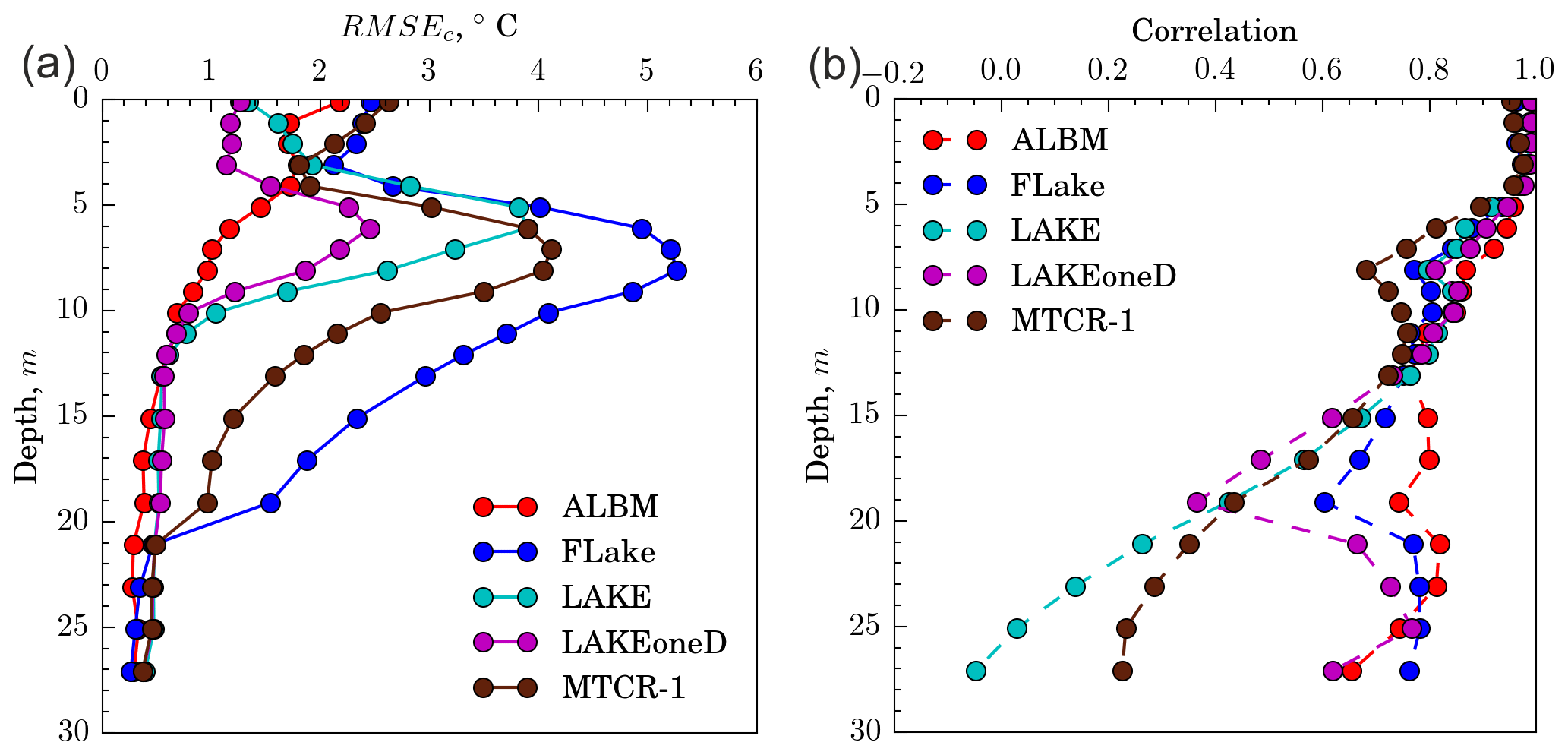
Figure 3(a) Centered root-mean-square error of modeled temperature calculated for each individual depth; (b) the correlation coefficient between the simulated and observed temperatures at each depth.
As highlighted in former studies (e.g., Stepanenko et al., 2010; Thiery et al., 2014b), this model overestimates the surface mixed-layer depth during summer, even under ice (Fig. 2b). The mixed-layer depth in the FLake model is 1.5 times larger than in observed data (5.6 m versus 3.6 m). Predictions of ice cover and ice off are characterized by large errors (see Table S3), with modeled dates more than 2 weeks off from the observations.
Remarkably, FLake demonstrates the largest sensitivity among all models to the lake depth – RMSEc is reduced approximately 2-fold (from 2.5 to 1.28 ∘C) (see Table S4, Figs. S3 and S4) when using a mean depth of 13.32 m instead of the maximal depth 37.5 m. The thickness of mixed-layer depth reduces up to 4.5 m and it has a better agreement with the observations in comparison with the RefSim experiment.
FLake showed a similar response in the sensitivity model test to variation of the light attenuation coefficient to other models. However, the difference in temperature is smaller than in other models: in both RefSim and ExtMinSim, ExtMaxSim is less than 4 ∘C in comparison with 8 ∘C (Fig. 4). It can be related to the weaker temperature gradient in the thermocline in comparison with other models (Fig. 2).
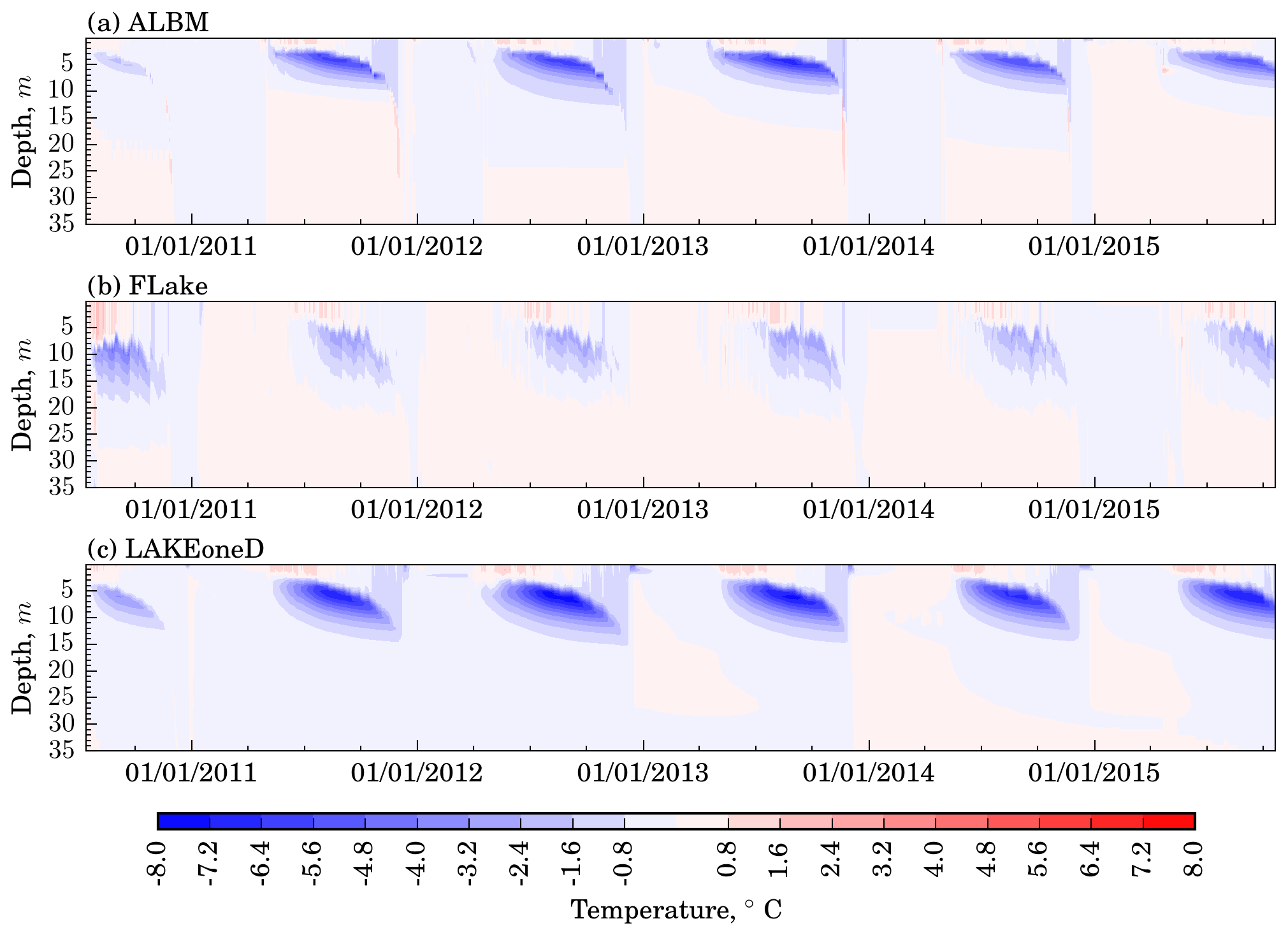
Figure 4Temperature difference between the ExtMaxSim and RefSim experiments in three lake models: (a) ALBM; (b) FLake; (c) LAKEoneD.
3.1.2 ALBM
The warmest model in terms of the epilimnion temperature was the ALBM (Fig. 2a). The maximum water temperature reached in the model is 32.4 ∘C (28.4 ∘C – in observations). However, the ALBM demonstrates the lowest RMSEc (1.53 ∘C) and the highest correlation (0.98) with the observed data for the temperature of the water column (except the surface) during the entire simulation period among all models (Figs. 3a and S2, Table S4). It can be noted visually that the shape of the thermocline is better reproduced by this model than by other model participants (Fig. 3a). In addition, the correlation coefficient of ALBM temperature decreases more slowly with depth than in all other models (Fig. 3b). In contrast, RMSEc for the surface temperature in the ALBM is almost 1.5 times larger than in k−ε models (see Fig. S2a, Table S4).
The ALBM successfully reproduces autumnal overturn, although the homogeneous temperature distribution in this model occurs approximately 7–10 d later compared to the measurements. The likely reason for this offset is the excessive accumulation of heat in the mixed layer during summer, which delays the cooling to the temperature of maximum density and subsequent vertical mixing.
The ice-cover and ice-off dates are quite close to observations (e.g., 24 December versus 28 December 2011; see Table S3). Differences between model and observation ice-cover dates of more than 2 weeks happen three times. The large errors mainly occur for ice cover, likely due to the excessive heat accumulated in summer.
3.1.3 MTCR-1 model
In terms of temperature, the Henderson-Sellers-based MTCR-1 model shows contrasting performance compared to ALBM (Fig. 2e). It is generally the coldest model (the temperature reaches a maximum of 24.2 ∘C in the epilimnion) and results in the deepest mixed layer (5.9 m versus 3.6 m observed). This significant difference in mixed-layer depth (see Table S2) is possibly associated with different schemes of convective mixing.
Similarly to the FLake model, the surface temperature in MTCR-1 is sensitive to changes in lake depth. The surface temperature DM reduced 4 times compared to the reference model simulation when decreasing the lake depth from 37.5 to 13.32 m (see Table S4).
While MTCR-1 and LAKEoneD use similar parameterization for ice formation and melt, their results are similar only for the ice-off dates. The ice-cover dates greatly vary between these models, with differences reaching up to 1 month (winter 2011–2012). Interestingly, LAKEoneD produces ice-melt periods in winters 2011–2012 and 2012–2013 (see Table S3), when MTCR-1 does not show it at all (there is no observed ice melt during these winters).
3.1.4 LAKEoneD and LAKE models
Even though LAKE and LAKEoneD use the same turbulence closure, they represent the temperature dynamics in the lake with considerable differences (Fig. 2c and d). In particular, the mean depth of the mixed layer as simulated by LAKE is 1 m deeper compared to LAKEoneD results (4.8 and 3.9 m, respectively). LAKE demonstrates greater heating of the epilimnion (up to 30 ∘C) than LAKEoneD (maximum value of 27.3 ∘C). The homogeneous distribution of temperature during autumn mixing predicted by LAKEoneD reaches the depth of 15 m in most years, as opposed to LAKE (up to 35 m) and the observational data (at least up to 25 m, where the deepest sensor is located). Remarkably, only in these two models do periods of unstable ice cover occur. For example, the ice in LAKE is thin and often comes off during winter (more than five times in winter 2011–2012), leading to wind-driven surface layer mixing (see Table S3).

Figure 5Time–depth distribution of the ED in Harp Lake (14 July 2010–19 October 2015), RefSim model experiment.
The sensitivity experiments with varying light attenuation coefficients (see Table S4) generally result in a similar response in all models. Increasing the light attenuation coefficient (i.e., reducing water transparency) leads to an upward shift of the thermocline position (Fig. 4); conversely, decreasing the attenuation coefficient causes a downward move of the thermocline. This leads to a temperature change at respective depths of up to 4 ∘C in the FLake model and 8 ∘C in the ALBM and LAKEoneD. Figure 4 contains only three models with different types of turbulent closure because the effect of varying the light attenuation coefficient is very similar in models of the same type (e.g., k−ϵ models LAKEoneD and LAKE).
It is important to note that all models have a maximum error, RMSEc for temperature (compared to observations) in the thermocline (Fig. 3a), which agrees with a previous study (Stepanenko et al., 2014). Conversely, the correlation between simulated and observed temperature decreases with depth in all models (Fig. 3b), starting from 0.9–1.0 near the surface to 0.1–0.7 close to the bottom.
3.2 Eddy diffusivity
Eddy diffusivity (ED), K, is the variable controlling the vertical turbulent transport in lake models. This section examines the results of simulated ED values, thereby focusing on discrepancies between models caused by different turbulent closure schemes.
The simulated time–depth distribution of ED is shown in Fig. 5. EDs in ALBM and MTCR-1 do not reproduce spring and autumn whole-water-column mixing as the Henderson-Sellers diffusivity is not valid for unstable stratification. In contrast, k−ε models correctly predict the deepening of the mixed layer in the ED pattern during summertime towards a complete mixing during autumn.
Even models employing the same type of turbulence parameterization differ in simulated eddy diffusivities in the thermocline by orders of magnitude. This is caused by the different background values of ED added to those estimated by turbulence closures and mimicking mixing mechanisms not directly resolved in 1-D models such as internal wave breaking (e.g., Hondzo and Stefan, 1993). Apparently, the background diffusivity is switched off in the MTCR-1 model during ice cover.
The increase in ED near the bottom during the stratified period in the ALBM can be explained by the change from a stable stratification in the thermocline to a quasi-neutral stratification beneath.
A peculiar feature of LAKE is that it features high-intensity turbulence during much of the ice-cover period in the lower part of the water column that is apparently related to residual flow after the autumn overturn. In contrast, in LAKEoneD, turbulence dissipates shortly after the ice cover. Both of these models demonstrate a subsurface region of high ED values in winter which is not reproduced by other models. Production of turbulent kinetic energy (TKE) below the ice may be caused by both momentum transfer through partial ice cover (implemented in LAKE) and shortwave radiation penetration causing under-ice convection. The conspicuous difference between LAKE and LAKEoneD results is that springtime deep mixing does not develop in LAKEoneD. This may be linked to different constants and stability functions used in its k−ε closures or different buoyancy and momentum fluxes at the lake–atmosphere interface during this season.
It is worth noting that the significant difference between the modeled and observed dates of ice cover and ice off (see Table S3) leads to errors in the simulation of ED as water opens and interacts with the atmosphere.
The main features of ED distribution over seasons described in this section hold in experiment LDSim with a different lake depth value (13.32 m).
3.3 Effects of eddy diffusivity on the vertical distribution of a passive tracer
The vertical distribution of ED in lake models is one of the major drivers of vertical transport of dissolved gases and their emission to the atmosphere. To isolate the effect of the ED parameterization in the different models, we solve the diffusion equation for a passive tracer concentration C:
The emission rate of the passive tracer at the bottom is set constant:
while at the surface the flux is assumed to be large enough to make the surface concentration negligible compared to deep-water concentration, so that the boundary condition here becomes
Setting zero concentration at the surface is justified by the fact that surface concentration of gases of interest (CO2, CH4) is typically orders of magnitude less than bottom concentration. The total (molecular plus turbulent) diffusivity K is taken from different models, so that the solution C of Eqs. (1–3) is individual for each lake model.
Calculation of tracer diffusion was carried out using simulated values K(z, t) from the two Henderson-Sellers-based models – ALBM, MTCR-1, and two k−ε models – LAKE and LAKEoneD, covering the period of 5 years. In order to take into account vertical mixing under unstable stratification performed in ALBM and MTCR-1 and not expressed by Henderson-Sellers diffusivity, a value K=105 m2 s−1 was applied for the convective layer in such cases.
The results of the numerical tracer experiment are presented in Fig. 6. All models demonstrate seasonal variability of the passive tracer concentration, including the near-bottom accumulation during stratified periods. Three models (ALBM, MTCR-1, and LAKE) perform the full overturn of the water column during autumn and spring, leading to the emission of almost the whole tracer storage to the atmosphere and forming a homogeneous concentration profile. In LAKEoneD, the vertical mixing does not reach the lake bottom during spring and autumn in certain years (e.g., 2011 and 2014). Hence, not all tracer amount is removed from the water column during overturn periods (see Fig. S5b) in this model. As a result, not only the concentration of the tracer near the bottom, but also the total tracer amount in the water column increases in LAKEoneD throughout the simulation period. However, this effect is a result of the assumption of a bathtub-shaped lake bathymetry and would be less when including the depth dependence of lake volume.
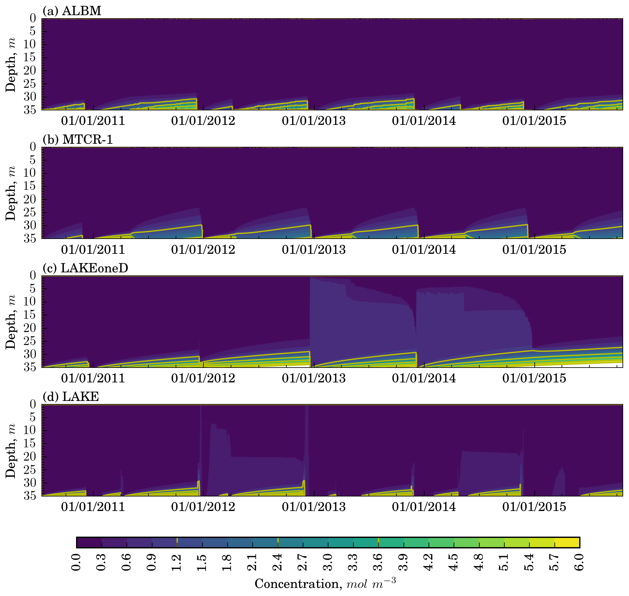
Figure 6Vertical distribution of passive tracer concentration in Harp Lake simulations, according to different models.
The MTCR-1 model demonstrates short overturn periods similar to those of LAKEoneD, but the mixing reaches deeper. Hence, the passive tracer does not accumulate over time. Furthermore, ALBM exhibits a higher near-bottom concentration than MTCR-1 because the ED simulated by ALBM is 1 order of magnitude lower compared to MTCR-1 at 30–35 m depth (see Fig. 6).
To assess the effect of different eddy diffusivities on the surface tracer flux, we use the ratio of the surface flux, Fsurf, to the bottom flux, Fbot, where the former is given as
with Ceq=0 the surface concentration, Cw the concentration at the first model output level below the surface (0.3 m), both in mol m−3, Δz=0.3 m, and Ksurf the surface diffusivity coefficient.
The Henderson-Sellers-based models produce short periods with high fluxes, primarily during autumnal mixing (see Fig. S5a), and the drops of the integral concentration in the water column at the same time (see Fig. S5b). The flux spikes are several orders of magnitude higher compared to k−ε models. A reasonable explanation is that instantaneous convective mixing implemented in the ALBM and MTCR-1 models leads to almost the whole tracer content inside the convective layer being released to the atmosphere during a single convective event. All the models demonstrate much weaker tracer fluxes during spring overturn compared to those resulting from autumnal convection.
Lake models with k−ε closure produce substantial tracer fluxes during the stratified period in particular years (e.g., 2013 and 2014). The likely reason for this effect is rapid changes in mixed-layer depth, due to sudden wind forcing, entraining higher concentrations from the hypolimnion into the mixed layer.
The tracer diffusion experiment was also conducted at the reduced depth of 13.32 m (see Fig. S5c and d). Due to the lower depth, seasonal vertical mixing now extends over the whole water column in all models, providing more effective release of the substance. ALBM and MTCR-1 demonstrate episodic high fluxes during summer along with k−ε models. The spring mixing in LAKEoneD now reaches the bottom in some years; hence, the integral tracer amount evolves here in a similar way compared to all other models. The time-averaged tracer emission in LAKEoneD is thus the most sensitive to depth reduction. The mean surface flux in this model increases up to approximately 54 %, while for the ALBM, MTCR-1, and LAKE this increase is 4 %, 19 %, and 8 %, respectively. This can be primarily explained by the contribution of the increased fluxes during summer stratification and of the autumn mixing now reaching the bottom.
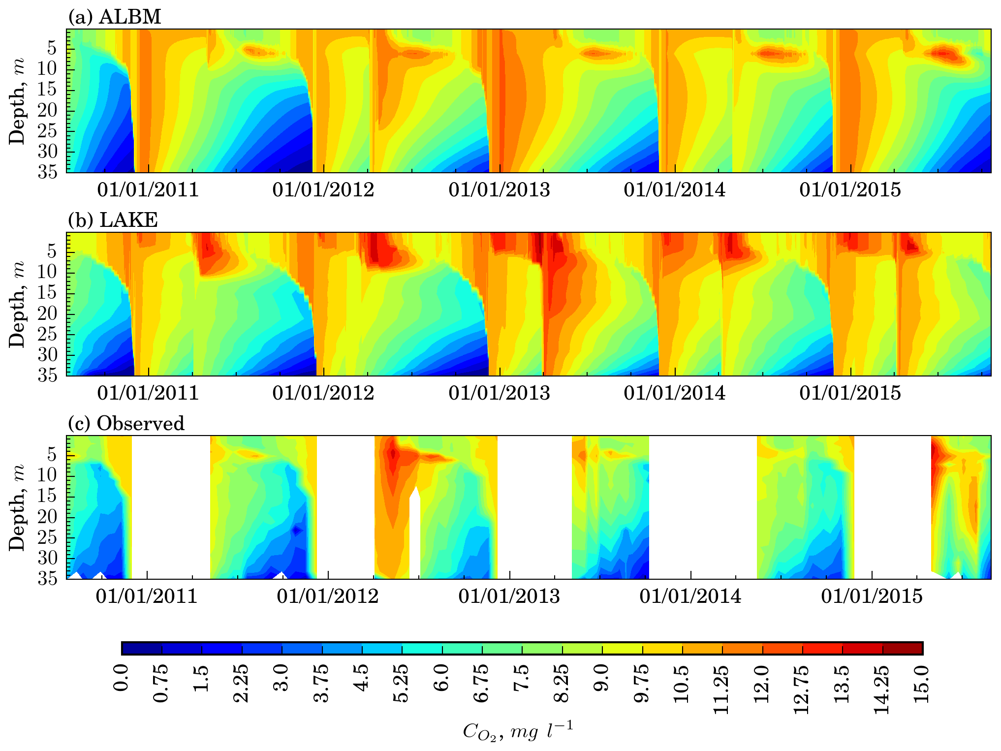
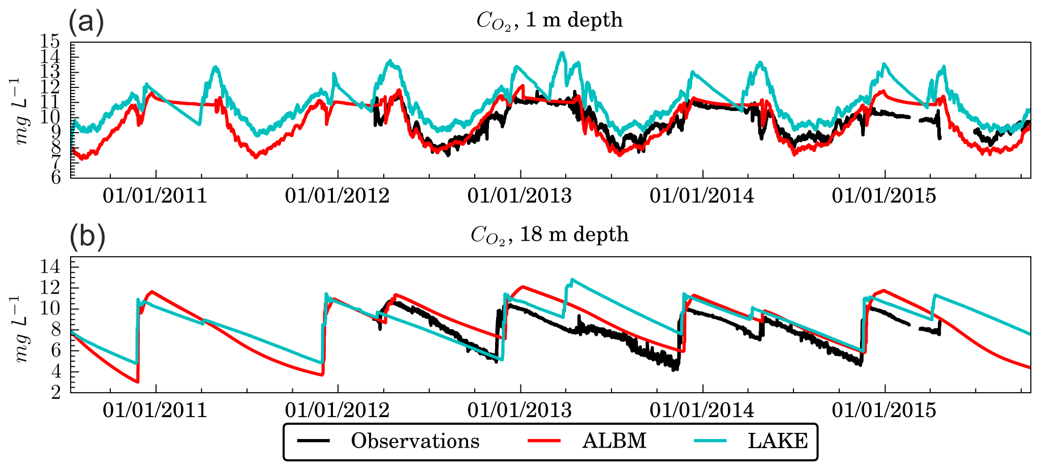
Figure 7Time–depth profiles of O2 in Harp Lake (14 July 2010–19 October 2015) and model experiment including sediments and morphometry (GasSim) for (a) ALBM and (b) LAKE. White patterns in (c) indicate absence of data.
3.4 Harp Lake biogeochemistry
3.4.1 Oxygen
The evolution of the observed vertical distribution of O2 concentration in Harp Lake is shown in Fig. 7c excluding winter periods and data with higher sampling frequency (1 h) collected at 1 and 18 m depth (Fig. 8). During spring (end of April–beginning of May) after ice off, convective mixing occurs, leading to a homogenized O2 profile. The similar process happens in autumn. During summer, O2 depletes in the hypolimnion due to its consumption by organic matter degradation in sediments and deep water layers. The main source of O2 is located in the photic layer, where it forms as a result of photosynthesis. Below the mixed layer (at 5–10 m depth), there is a maximum of O2 concentration due to weak turbulence, so that the produced O2 is not transported to the surface and is eventually emitted to the atmosphere. Emergence of this maximum is consistent with observations of a number of other freshwater lakes (Camacho, 2006; Cantin et al., 2011). In particular, the O2 maximum is remarkable during the summer of 2012: increases up to 15 mg L−1 at 5 m depth. During winter, the O2 concentration is usually high, indicating a relatively low O2 consumption rate from organic matter degradation in the lake. In summer, surface oxygen content decreases following reduction of temperature-controlled solubility. The measurements thus indicate common trends observed in most deep oligotrophic lakes at mid-latitudes (Mitchell and Prepas, 1990).
Both models depict a reasonable representation of O2 dynamics at different depths (Fig. 7a and b). The ALBM includes the O2 model described in Tan et al. (2017), whereas LAKE employs the representation of O2 sinks and sources from Stefan and Fang (1994). Even though they use different oxygen and turbulent parameterizations, both models show a similar spatiotemporal pattern. In particular, they reproduce the maximum of O2 concentration below the mixed layer, its quasi-linear in time decrease in the hypolimnion (18 m) during stratified periods, and the effect of mixing events during spring and autumn, marked by rapid changes in O2 concentration at 18 m depth. However, the O2 concentration as computed by LAKE is on average 1–2 mg L−1 higher than the observed values. A plausible explanation for this positive bias is that photosynthesis in LAKE yields excessive production of O2 (parameters of biogeochemical parameterizations in this model have not been calibrated in the study). Another deficiency of LAKE simulations is that during ice cover near-surface O2 decays linearly and then exhibits significant peaks at thinning of ice cover and ice off, whereas in the ALBM and measurements, oxygen content remains almost constant during these periods, which is more consistent with measurements.
The time series of O2 concentration from the ALBM and LAKE correlate reasonably with observed data, with the linear correlation coefficient ranging between 0.5 and 0.6 at 1 m and between 0.6 and 0.8 at 18 m depth, and with RMSEc 1.27–1.56 mg L−1 at 1 m and 1.19–1.52 at 18 m depth (see Fig. S6). For both depths, the ALBM demonstrates higher correlation with observations. Both models correlate better with observations at large depth. Decrease in the temperature in the ExtMaxSim simulation (Fig. 4) due to the upward shift of the thermocline leads to the reduction of O2 concentrations at the respective depths due to temperature dependence of photosynthesis.
Overall, the oxygen content is highly dependent on physical controls, which are temperature, radiation, ED and ice cover. Given that these factors are reasonably reproduced by the ALBM and LAKE, the O2 spatiotemporal pattern is captured as well. Successful representation of maximal O2 content below the mixed layer during summer may be an important modeling skill for simulating correctly CH4 in a lake because the former acts as a sink region for the latter. Furthermore, realistic oxygen concentration reduction during periods of stable stratification means that the respective CO2 production from aerobic organic matter decomposition is reproduced reasonably as well.
3.4.2 Carbon dioxide
The vertical distributions of CO2 concentrations simulated by the ALBM and LAKE are shown in Fig. 9. The ALBM simulates higher concentrations of CO2 compared to LAKE. This is likely because, in contrast to LAKE, the ALBM considers dissolved inorganic carbon (DIC) inflow from the catchment and explicitly treats DOC and particulate organic carbon (POC) dynamics (Tan et al., 2017). Parameter calibration applied in the ALBM brought CO2 content closer to measurements in this model. Correlation with the observational data at a depth of 0.39 m is relatively small for both models (0.3), and RMSEc is 4.5 and 2.7 mg L−1 for LAKE and the ALBM, respectively.
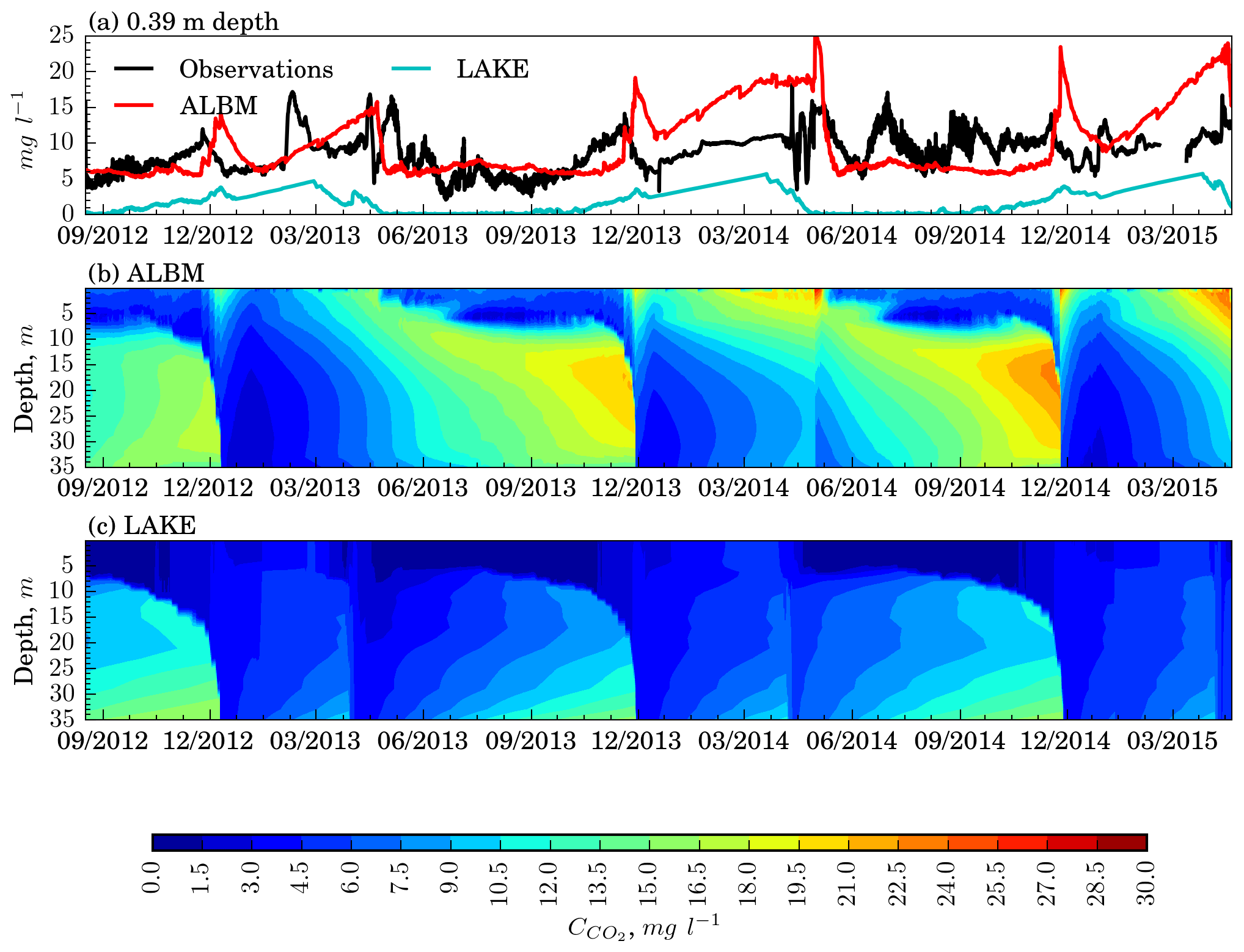
Figure 9Time–depth profiles of CO2 concentration in Harp Lake (17 August 2012–20 April 2015), experiment including modules of sediments and morphometry (GasSim).
Both models reproduce the seasonality of the CO2 concentrations: during summer CO2 accumulates in the hypolimnion, while CO2 is consumed in the mixed layer due to photosynthesis. For the same reason, the depth of the O2 maximum (Fig. 7c) is consistent with the metalimnetic CO2 minimum.
Vertical turbulent diffusion (Sect. 3.3) greatly affects CO2 patterns in models. In particular, the mixing periods clearly seen in Fig. 9 coincide with those in Fig. 6. Accumulation of CO2 below the mixed layer during stratified periods is clearly demonstrated by both models. However, the vertical CO2 distribution in the thermocline is very different; i.e., in LAKE, concentration attains its maximum near the bottom, whereas in the ALBM the maximum is located at 15–20 m depth. This can be related to the fact that in the ALBM, DOC and DIC from surface water and groundwater can be injected in the middle of the water column.
In contrast to oxygen, measured CO2 content is much less correlated with simulated series. The wintertime increase in surface concentration seen in calculated series is hardly observable in measured data. In summer, simulated CO2 series are smooth, whereas there are significant fluctuations in empirical data. There is some correspondence between seasonal-mixing-caused peaks in modeled concentration and the measured one, though with time lags. All this leads to the conclusion that, compared to oxygen, carbon dioxide is more controlled by biogeochemical processes misrepresented in lake models than by physical factors. As stated in the previous section, a realistic decay of oxygen content during stratified periods in the ALBM and LAKE models suggests that CO2 amount produced by aerobic decomposition of organic matter in both the water column and in the top part of sediments is reasonably simulated as well. Satisfactory agreement of computed oxygen in the mixed layer and below with observations implies that photosynthesis minus respiration rate is fairly captured as well, and so do the models for CO2 gain or loss due to these processes. Hence, the primary drawback of the models used in respect to DIC simulation is likely to be not explicitly simulating transport of carbon species from catchment to a water body. Thus, modeling approaches coupling the catchment and a lake presented recently (Futter et al., 2008; Duffy et al., 2018; McCullough et al., 2018) should be elaborated and used more widely.
The important role of catchment processes in building up the DIC levels in lakes introduces an extra difficulty for implementing lacustrine CO2 emissions in the Earth system models. This is caused by the necessity to provide regional or global data on a lake catchment's geometric, physical and biogeochemical properties, which are not currently available. In relation to this, we can also note a faster progress on a roadmap to introduce lake CH4 dynamics in climate models, where simulations passed from site-level studies to regional estimates (Tan et al., 2015), whereas CO2 modeling is currently confined to individual lakes (Stepanenko et al., 2016; Tan et al., 2017; Kiuru et al., 2018).
A lake model intercomparison study focusing on physical controls of biogeochemical species (i.e., dissolved gas concentration) is performed, marking a step forward in the LakeMIP exercises, which have been previously focused on thermodynamic modeling only. To evaluate model performance with respect to biogeochemical processes, we had to first evaluate their performance in hydrodynamic/thermodynamic simulations and variations due to uncertainty in major driving parameters, such as temperature and turbulent diffusivity.
The participating lake models (ALBM, FLake, LAKE, LAKEoneD, MTCR-1) were evaluated regarding their ability to reproduce the thermodynamic regime of Harp Lake. All the models capture the seasonal variability of the temperature profile in the deep boreal dimictic lake. A substantial discrepancy was found between the models in the representation of thermocline evolution – consistent with previous studies – and the correlation coefficient for calculated and observed temperature was found to decrease from surface to bottom (from 0.9–1 to 0.1–0.6). The sensitivity of the simulation results to the light attenuation coefficient and the lake depth was assessed, given that in global applications, such as numerical weather prediction, they are external parameters known with high uncertainty.
All considered lake models do not accurately reproduce the dates of ice cover and ice off, similar to the results from a previous simulation study for the same lake which used other lake models and an earlier time period (Yao et al., 2014). The difference between the model results and the observations exceeds 2 weeks in particular years. The unrealistic representation of ice formation and ice melt dates leads to untimely changes in eddy diffusivity (ED) within the water column, which in turn strongly affects the modeled distribution of gases and their emission to the atmosphere. This implies more efforts of a community should be spent on elaborating ice–snow schemes in lake models, where currently vertical homogeneity and temporal invariance of optical and thermodynamic properties are typically assumed, which does not correspond to a bulk of existing knowledge (Leppäranta, 2015). In a recent study (Tan et al., 2018), one possible direction to improve the simulation of ice cover is shown. They demonstrated that including the conversion of snow to white or slush ice when the weight of ice and snow exceeds the buoyancy of the ice cover can significantly improve the ice simulation results. In the special case of saline lakes, effects of salt trapping in ice cover become important and should be adequately parameterized as well (Stepanenko et al., 2019).
To study the effect of turbulent transport on the vertical distribution of gases, we conducted passive tracer simulations using simulated ED from different models.
This experiment reveals that all lake models demonstrate more intense mixed-layer deepening during autumn than during spring, with spring overturn in some cases not even reaching the lake bottom (e.g., in MTCR-1 and LAKEoneD).
Moreover, less intensive mixing during spring and autumn leads to an accumulation of passive tracer concentrations in deep water at a multiyear timescale.
In addition, the representation of an equivalent lake depth in 1-D models is found to be a crucial parameter regulating both passive tracer concentration and its flux to the atmosphere: when reducing the depth of a lake approximately by 50 %, the average tracer flux increased by 4 %–54 %.
The lake models with the most comprehensive biogeochemical modules, such as ALBM and LAKE, demonstrated reasonable reproduction of the O2 concentration profile and its seasonal evolution. For instance, both models predict an oxygen concentration maximum and corresponding CO2 minimum below the mixed layer in summer, elevated surface concentration and linear decay of deep-water content under ice cover, and vertical homogenization during spring and autumn overturns.
The main difference between the models in the CO2 simulation is that the ALBM involves an additional source of DIC from the catchment. Due to this, the average CO2 concentration in the ALBM is higher than in LAKE and closer to measurements. Results from both models are weakly correlated with measurements of surface CO2 concentration. This leads to the conclusion that, compared to oxygen, carbon dioxide is much more controlled by biogeochemical processes misrepresented in lake models than by physical factors.
As a result of this study, we emphasize the following issues to be addressed by the lake modeling community in respect to dissolved gas simulation.
-
Simplified lake modeling approaches especially employing a parameterized temperature profile and representing reasonably the surface temperature may fail in calculating vertical temperature distribution, with a potentially significant effect on biogeochemical processes if the respective module is coupled to the thermodynamic compartment.
-
For deep lakes, models differ in the depth of autumn and especially spring overturn; if this depth reaches bottom, the gas content originating from sediments and accumulating in the hypolimnion during the preceding stratified period is almost completely released to the atmosphere; otherwise, these gases may continuously accumulate in deep water at a multi-year timescale; however, more research is needed to establish the effect of lake morphometry on these processes.
-
Oxygen content in both surface and deep water is efficiently controlled by physical and biogeochemical factors, successfully simulated by lake models, whereas measured surface CO2 exhibits significant temporal variability not captured by the models, calling for more research in biogeochemical mechanisms and parameterizations of carbon dioxide dynamics.
-
1-D models have certain limitations when applied to such a 3-D system as a lake. They do not capture all the lake mixing mechanisms such as density-driven currents, which can be important under certain conditions (Samolyubov, 1999). It was found that for deep lakes with an extended littoral zone such as Lake Geneva (Fer et al., 2001, 2002) or Lake Van (Kaden et al., 2010), these flows can be significant in terms of vertical heat and gas transfer. In particular, for Harp Lake it may be not important due to smaller depth and not a large shallow area. In winter, a large-scale convective circulation (up to 3–5 cm s−1) due to heat exchange at the sediment–water interface may develop under ice (Kirillin et al., 2015). However, the importance of this circulation in terms of gas transfer has not been studied yet. So far, to the best of our knowledge, these currents are not parameterized in 1-D models.
-
ALBM: available upon request to Zeli Tan, e-mail tanzeli1982@gmail.com;
-
MTCR-1: available upon request to Bruna Arcie Polli, e-mail brunapolli@gmail.com;
-
FLake; publicly available at the website http://www.flake.igb-berlin.de/ (last access: 16 February 2020; Mironov et al., 2020);
-
LAKEoneD: available upon request to Klaus Jöhnk, e-mail science@limnophysics.de;
-
LAKE: publicly available at the website http://tesla.parallel.ru/Viktor/LAKE/wikis/LAKE-model (last access: 16 February 2020; Stepanenko and Debolskiy, 2019;
-
Observational data: available upon request to Huaxia Yao, e-mail huaxia.yao@ontario.ca.
The supplement related to this article is available online at: https://doi.org/10.5194/hess-24-697-2020-supplement.
VS, WT, KJ, ZT, and HY conceptually designed the experiments. SG, BAP, TB, WT, KJ, ZT, and QZ carried them out and provided the results of the simulations. JAR and HY provided observational data. SG made a formal analysis and combined all the data and visualized them under the supervision of VS. SG prepared the manuscript under the supervision of AL and VS with significant contributions from all the co-authors.
The authors declare that they have no conflict of interest.
This article is part of the special issue “Modelling lakes in the climate system (GMD/HESS inter-journal SI)”. It is a result of the 5th workshop on “Parameterization of Lakes in Numerical Weather Prediction and Climate Modelling”, Berlin, Germany, 16–19 October 2017.
Zeli Tan is supported by the US DOE's Earth System Modeling program through the Energy Exascale Earth System Model (E3SM) project. The supercomputing resource for ALBM simulations is provided by the Rosen Center for Advanced Computing at Purdue University. The Uniscientia Foundation and the ETH Zurich Foundation are acknowledged for their support to this research. Thanks are given to DESC staff (in particular Ron Ingram, Chris McConnell, and Tim Field) for contributing to data collection and to the Ontario Ministry of the Environment and Climate Change for funding the traditional and high-frequency lake monitoring activities. Simulations of MTCR-1 were supported by the Brazilian funding agencies CNPQ (grant no. 308758/2017-0) and CAPES.
This research has been supported by the Russian Science Foundation (grant no. 17-17-01210), the USGS project (grant no. G17AC00276), the ETH Zurich postdoctoral fellowship (grant no. Fel-45 15-1), and the CNPQ (grant no. 308758/2017-0).
This paper was edited by Miguel Potes and reviewed by two anonymous referees.
Ashton, G. D.: Freshwater ice growth, motion and decay, in: Dynamics of Snow and Ice Masses, edited by: Colbeck, S., Academic Press, New York, 261–304, 1980. a, b, c
Ashton, G. D.: River and lake ice thickening, thinning and snow ice formation, Cold Reg. Sci. Technol., 68, 3–19, https://doi.org/10.1016/j.coldregions.2011.05.004, 2011. a, b, c
Balsamo, G., Dutra, E., Stepanenko, V. M., Viterbo, P., Miranda, P., and Mironov, D.: Deriving an effective lake depth from satellite lake surface temperature data: a feasibility study with MODIS data, Boreal Environ. Res., 15, 178–190, https://doi.org/10.21957/be525ccu, 2010. a
Bastviken, D., Tranvik, L. J., Downing, J. A., Crill, P. M., and Enrich-Prast, A.: Freshwater methane emissions offset the continental carbon sink, Science, 331, 50, https://doi.org/10.1126/science.1196808, 2011. a
Camacho, A.: On the occurrence and ecological features of deep chlorophyll maxima (DCM) in Spanish stratified lakes, Limnetica, 25, 453–478, 2006. a
Cantin, A., Beisner, B. E., Gunn, J. M., Prairie, Y. T., Winter, J. G.: Effects of thermocline deepening on lake plankton communities, Can. J. Fish. Aquat., 68, 260–276, 2011. a
Choulga, M., Kourzeneva, E., Zakharova, E., and Doganovsky, A.: Estimation of the mean depth of boreal lakes for use in numerical weather prediction and climate modeling, Tellus A, 66, 21295, https://doi.org/10.3402/tellusa.v66.21295, 2014. a
Cox, E. T.: Counts and Measurements of Ontario Lakes: Watershed Unit Summaries Based on Maps of Various Scales by Wathershed Unit, Ontario Ministry of Natural Resourses, Toronto, Ontario, Canada, 1978. a
Dillon, P. J., Reid, R. A., and De Grosbois, E.: The rate of acidification of aquatic ecosystems in Ontario, Canada, Nature, 329, 45–48, 1987. a, b
Docquier, D., Thiery, W., Lhermitte, S., and Van Lipzig, N.: Multi-year wind dynamics around Lake Tanganyika, Clim. Dynam., 47, 3191–3202, https://doi.org/10.1007/s00382-016-3020-z, 2016. a
Duffy, C. J., Dugan, H. A., and Hanson, P. C.: The age of water and carbon in lake-catchments: A simple dynamical model, Limnol. Oceanogr. Lett., 3, 236–245, https://doi.org/10.1002/lol2.10070, 2018. a
Fang, X. and Stefan, H. G.: Temperature and dissolved oxygen simulations for a lake with ice cover, Project Report 356, St. Anthony Falls Hydraulic Laboratory, University of Minnesota, Minneapolis, MN, 65 pp., 1994. a, b
Fang, X. and Stefan, H. G.: Long-term lake water temperature and ice cover simulations/measurements, Cold Reg. Sci. Technol., 24, 289–304, 1996. a
Fer, I., Lemmin, U., and Thorpe, S. A.: Cascading of water down the sloping sides of a deep lake in winter, Geophys. Res. Lett., 28, 2093–2096, https://doi.org/10.1029/2000GL012599, 2001. a
Fer, I., Lemmin, U., and Thorpe, S. A.: Winter cascading of cold water in Lake Geneva, J. Geophys. Res.-Oceans, 107, 3060, https://doi.org/10.1029/2001JC000828, 2002. a
Forbes, G. S. and Meritt, J. H.: Mesoscale vortices over the Great Lakes in wintertime, Mon. Weather Rev., 112, 377–381, 1984. a
Futter, M. N., Starr, M., Forsius, M., and Holmberg, M.: Modelling the effects of climate on long-term patterns of dissolved organic carbon concentrations in the surface waters of a boreal catchment, Hydrol. Earth Syst. Sci., 12, 437–447, https://doi.org/10.5194/hess-12-437-2008, 2008. a
Goudsmit, G. H., Burchard, H., Peeters, F., and Wüest, A.: Application of k−ε turbulence models to enclosed basins: The role of internal seiches, J. Geophys. Res.-Oceans, 107, 3230, https://doi.org/10.1029/2001JC000954, 2002. a
Heiskanen, J. J., Mammarella, I., Ojala, A., Stepanenko, V., Erkkilá, K. M., Miettinen, H., and Vesala, T.: Effects of water clarity on lake stratification and lake‐atmosphere heat exchange, J. Geophys. Res.-Atmos., 120, 7412–7428, https://doi.org/10.1002/2014JD022938, 2015. a
Henderson-Sellers, B.: New formulation of eddy diffusion thermocline models, Appl. Math. Model, 9, 441–446, 1985. a, b
Hondzo, M. and Stefan, H. G.: Lake water temperature simulation model, J. Hydraul. Eng., 119, 1251–1273, 1993. a
Hostetler, S. W. and Bartlein, P. J.: Simulation of lake evaporation with application to modeling lake level variations of Harney-Malheur Lake, Oregon, Water Resour. Res., 26, 2603–2612, 1990. a, b
Hostetler, S. W., Bates, G. T., and Giorgi, F.: Interactive coupling of a lake thermal model with a regional climate model, J. Geophys. Res.-Atmos., 98, 5045–5057, 1993. a
Jammet, M., Crill, P., Dengel, S., and Friborg, T.: Large methane emissions from a subarctic lake during spring thaw: Mechanisms and landscape significance, J. Geophys. Res.-Biogeo., 120, 2289–2305, https://doi.org/10.1002/2015JG003137, 2015. a
Jöhnk, K. D. and Umlauf, L.: Modeling the metalimnetic oxygen minimum in a medium sized alpine lake, Ecol. Model., 136, 67–80, https://doi.org/10.1016/S0304-3800(00)00381-1, 2001. a, b
Jöhnk, K. D., Huisman, J. E. F., Sharples, J., Sommeijer, B. E. N., Visser, P. M., and Stroom, J. M.: Summer heatwaves promote blooms of harmful cyanobacteria, Global Change Biol., 14, 495–512, https://doi.org/10.1111/j.1365-2486.2007.01510.x, 2008. a, b
Kaden, H., Peeters, F., Lorke, A., Kipfer, R., Tomonaga, Y., and Karabiyikoglu, M.: Impact of lake level change on deep‐water renewal and oxic conditions in deep saline Lake Van, Turkey, Water Resour. Res., 46, W11508, https://doi.org/10.1029/2009WR008555, 2010. a
Karlsson, J., Giesler, R., Persson, J., and Lundin, E.: High emission of carbon dioxide and methane during ice thaw in high latitude lakes, Geophys. Res. Lett., 40, 1123–1127, https://doi.org/10.1002/grl.50152, 2013. a
Kirillin, G. B., Forrest, A. L., Graves, K. E., Fischer, A., Engelhardt, C., and Laval, B. E.: Axisymmetric circulation driven by marginal heating in ice‐covered lakes, Hydrol. Geophys. Res. Lett., 42, 2893–2900, https://doi.org/10.1002/2014GL062180, 2015. a
Kirillin, G. B., Wen, L., and Shatwell, T.: Seasonal thermal regime and climatic trends in lakes of the Tibetan highlands, Hydrol. Earth Syst. Sci., 21, 1895–1909, https://doi.org/10.5194/hess-21-1895-2017, 2017. a
Kiuru, P., Ojala, A., Mammarella, I., Heiskanen, J., Kämäräinen, M., Vesala, T., and Huttula, T.: Effects of climate change on CO2 concentration and efflux in a humic boreal lake: A modeling study, J. Geophys. Res.-Biogeo., 123, 2212–2233, https://doi.org/10.1029/2018JG004585, 2018. a
Kourzeneva, E.: External data for lake parameterisation in Numerical Weather Prediction and climate modeling, Boreal Environ. Res., 15, 165–177, 2010. a
Lehner, B. and Döll, P.: Development and validation of a global database of lakes, reservoirs and wetlands, J. Hydrol., 296, 1–22, https://doi.org/10.1016/j.jhydrol.2004.03.028, 2004. a
Leppäranta, M.: Freezing of lakes and the evolution of their ice cover: Springer, Heidelberg, New York, Dordrecht, London, p. 301, https://doi.org/10.1007/978-3-642-29081-7, 2015. a
Long, Z., Perrie, W., Gyakum, J., Caya, D., and Laprise, R.: Northern lake impacts on local seasonal climate, J. Hydrometeorol., 8, 881–896, https://doi.org/10.1175/JHM591.1, 2007. a
Mahrt L.: Surface heterogeneity and vertical structure of the boundary layer, Bound.-Lay. Meteorol., 96, 33–62, https://doi.org/10.1023/A:1002482332477, 2000. a
McCullough, I. M., Dugan, H. A., Farrell, K. J., Morales-Williams, A. M., Ouyang, Z., Roberts, D., Scordo, F., Bartlett, S. L., Burke, S. M., Doubek, J. P., Krivak-Tetley, F. E., Skaff, N. K., Summers, J. C., Weathers, K. C., and Hanson, P. C.: Dynamic modeling of organic carbon fates in lake ecosystems, Ecol. Model., 386, 71–82, https://doi.org/10.1016/j.ecolmodel.2018.08.009, 2018. a
Mironov, D. V.: Parameterisation of lakes in numerical weather prediction. Part 1: Description of a lake model, available from the author, Dmitrii Mironov@dwd.de., 2003. a, b
Mironov, D. V.: Parameterisation of lakes in numerical weather prediction. Description of a lake model, COSMO Technical Report 11, Deutscher Wetterdienst, Offenbach am Main, Germany, 2008. a, b
Mironov, D., Terzhevik, A., Kirillin, G., and Simoncelli, S.: FLake model website, available at: http://www.flake.igb-berlin.de/, last access: 16 February 2020. a
Mitchell, P. and Prepas, E. E. (Eds.): Atlas of Alberta lakes, The University of Alberta Press, Edmonton, 1990. a
Molot, L. A. and Dillon, P. J.: Nitrogen/phosphorus ratios and the prediction of chlorophyll in phosphorus-limited lakes in central Ontario, Can. J. Fish. Aquat. Sci., 48, 140–145, 1991. a
Perroud, M., Goyette, S., Martynov, A., Beniston, M., and Anneville, O.: Simulation of multiannual thermal profiles in deep Lake Geneva: a comparison of one-dimensional lake models, Limnol. Oceanogr.-Meth., 54, 1574–1594, https://doi.org/10.4319/lo.2009.54.5.1574, 2009. a
Phelps, A. R., Peterson, K. M., and Jeffries, M. O.: Methane efflux from high‐latitude lakes during spring ice melt, J. Geophys. Res.-Atmos., 103, 29029–29036, https://doi.org/10.1029/98JD00044, 1998. a
Polli, B. A. and Bleninger, T.: Modelagem do transporte de calor no reservatório Vossoroca, in: 21 Simpósio Brasileiro De Recursos Hídricos, 22–27 November 2015, Federal District, Brasilia, Brazil, 1–8, 2015. a
Polli, B. A. and Bleninger, T.: Reservoir 1D heat transport model, J. Appl. Water Eng. Res., 1, 1–16, https://doi.org/10.1080/23249676.2018.1497560, 2018. a
Poole, H. H. and Atkins, W. R. G.: Photo-electric measurements of submarine illumination throughout the year, J. Mar. Biol. Assoc. UK, 16, 297–324, 1929. a
Raymond, P. A., Hartmann, J., Lauerwald, R., Sobek, S., McDonald, C., Hoover, M., Butman, D., Striegl, R., Mayorga, E., Humborg, C., Kortelainen, P., Dürr, H., Meybeck, M., Ciais, P., and Guth, P.: Global carbon dioxide emissions from inland waters, Nature, 503, 355–359, https://doi.org/10.1038/nature12760, 2013. a
Samolyubov, B. I.: Bottom stratified currents, Nauchny Mir, Moscow, 464 pp., 1999. a
Shatwell, T., Adrian, R., and Kirillin, G.: Planktonic events may cause polymictic-dimictic regime shifts in temperate lakes, Sci. Rep.-UK, 6, 24361, https://doi.org/10.1038/srep24361, 2016. a
Stefan, H. G. and Fang, X.: Dissolved oxygen model for regional lake analysis, Ecol. Model., 71, 37–68, https://doi.org/10.1016/0304-3800(94)90075-2, 1994. a
Stepanenko, V. M. and Debolskiy, A. V.: LAKE model website, available at: http://tesla.parallel.ru/Viktor/LAKE/wikis/LAKE-model, last access: 16 February 2020. a
Stepanenko, V. M., and Lykossov, V. N.: Numerical modeling of heat and moisture transfer processes in a system lake-soil, Russ. Meteorol. Hydrol., 3, 95–104, 2005. a, b
Stepanenko, V. M., Goyette, S., Martynov, A., Perroud, M., Fang, X., and Mironov, D.: First steps of a Lake Model Intercomparison Project: LakeMIP, Boreal Environ. Res., 15, 191–202, 2010. a, b, c, d
Stepanenko, V. M., Machulskaya, E. E., Glagolev, M. V., and Lykossov, V. N.: Numerical modeling of methane emissions from lakes in the permafrost zone, Izv. Atmos. Ocean Phys., 47, 252–264, https://doi.org/10.1134/S0001433811020113, 2011. a, b, c
Stepanenko, V. M., Jöhnk, K. D., Machulskaya, E., Perroud, M., Subin, Z., Nordbo, A., Mammarella, I., and Mironov, D.: Simulation of surface energy fluxes and stratification of a small boreal lake by a set of one-dimensional models, Tellus A, 66, 21389, https://doi.org/10.3402/tellusa.v66.21389, 2014. a, b
Stepanenko, V. M., Mammarella, I., Ojala, A., Miettinen, H., Lykosov, V., and Vesala, T.: LAKE 2.0: a model for temperature, methane, carbon dioxide and oxygen dynamics in lakes, Geosci. Model Dev., 9, 1977–2006, https://doi.org/10.5194/gmd-9-1977-2016, 2016. a, b, c, d
Stepanenko, V. M., Repina, I. A., Ganbat, G., and Davaa, G.: Numerical simulation of ice cover of saline lakes, Izv. Atmos. Ocean Phys., 55, 129–138, https://doi.org/10.1134/S0001433819010092, 2019. a
Subin, Z. M., Riley, W. J., and Mironov, D.: An improved lake model for climate simulations: model structure, evaluation, and sensitivity analyses in CESM1, J. Adv. Model Earth Syst., 4, M02001, https://doi.org/10.1029/2011MS000072, 2012. a
Tan, Z. and Zhuang, Q.: Arctic lakes are continuous methane sources to the atmosphere under warming conditions, Environ. Res. Lett., 10, 054016, https://doi.org/10.1088/1748-9326/10/5/054016, 2015. a, b
Tan, Z., Zhuang, Q., and Walter Anthony, K.: Modeling methane emissions from arctic lakes: Model development and site level study, J. Adv. Model Earth Syst., 7, 459–483, https://doi.org/10.1002/2014MS000344, 2015. a, b
Tan, Z., Zhuang, Q., Shurpali, N. J., Marushchak, M. E., Biasi, C., Eugster, W., and Walter Anthony, K.: Modeling CO2 emissions from Arctic lakes: Model development and site‐level study, J. Adv. Model Earth Syst., 9, 2190–2213, https://doi.org/10.1002/2017MS001028, 2017. a, b, c, d, e
Tan, Z., Yao, H., and Zhuang, Q.: A small temperate lake in the 21st century: Dynamics of water temperature, ice phenology, dissolved oxygen and chlorophyll-a, Water Resour. Res., 54, 4681–4699, https://doi.org/10.1029/2017WR022334, 2018. a, b
Thiery, W., Stepanenko, V. M., Fang, X., Jöhnk, K. D., Li, Z., Martynov, A., Perroud, M., Subin, Z. M., Darchambeau, F., Mironov, D., and Van Lipzig, N. P.: LakeMIP Kivu: evaluating the representation of a large, deep tropical lake by a set of one-dimensional lake models, Tellus A, 66, 21390, https://doi.org/10.3402/tellusa.v66.21390, 2014a. a, b, c
Thiery, W., Martynov, A., Darchambeau, F., Descy, J. P., Plisnier, P. D., Sushama, L., and van Lipzig, N. P.: Understanding the performance of the FLake model over two African Great Lakes, Geosci. Model Dev., 7, 317–337, https://doi.org/10.5194/gmd-7-317-2014, 2014b. a
Thiery, W., Davin, E. L., Panitz, H.-J., Demuzere, M., Lhermitte, S., and Lipzig, N.: The Impact of the African Great Lakes on the Regional Climate, J. Climat, 28, 4061–4085, https://doi.org/10.1175/JCLI-D-14-00565.1, 2015. a, b
Thiery, W., Davin, E. L., Seneviratne, S. I., Bedka, K., Lhermitte, S., and van Lipzig, N. P.: Hazardous thunderstorm intensification over Lake Victoria, Nat. Commun., 7, 12786, https://doi.org/10.1038/ncomms12786, 2016. a
Thiery, W., Gudmundsson, L., Bedka, K., Semazzi, F. H., Lhermitte, S., Willems, P., Van Lipzig, N. P., and Seneviratne, S. I.: Early warnings of hazardous thunderstorms over Lake Victoria, Environ. Res. Lett., 12, 074012, https://doi.org/10.1088/1748-9326/aa7521, 2017. a
Tranvik, L. J., Downing, J. A., Cotner, J. B., Loiselle, S. A., Striegl, R. G., Ballatore, T. J., Dillon, P., Finlay, K., Fortino, K., Knoll, L. B., Kortelainen, P. L., Kutser, T., Larsen, S., Laurion, I., Leech, D. M., McCallister, S. L., McKnight, D. M., Melack, J. M., Overholt, B. S., Porter, J. A., Prairie, Y., Renwick, W. H., Roland, F., Sherma, B. S., Schindler, D. W., Sobeck, S., Tremblay, A., Vanni, M. J., Verschoor, A. M., von Wachenfeldt, E., and Weyhenmeyer, G. A.: Lakes and reservoirs as regulators of carbon cycling and climate, Limnol. Oceanogr., 54, 2298–2314, https://doi.org/10.1029/2000JD900719, 2009. a
Wik, M., Varner, R. K., Anthony, K. W., MacIntyre, S., and Bastviken, D.: Climate-sensitive northern lakes and ponds are critical components of methane release, Nat. Geosci., 9, 99–105, https://doi.org/10.1038/ngeo2578, 2016. a
Yao, H., Samal, N. R., Joehnk, K. D., Fang, X., Bruce, L. C., Pierson, D. C., Rusak, J. A., and James, A.: Comparing ice and temperature simulations by four dynamic lake models in Harp Lake: past performance and future predictions, Hydrol. Process., 28, 4587–4601, https://doi.org/10.1002/hyp.10180, 2014. a, b