2.1 Study site and data

The study site is a 10.2 ha catchment in the city of Luleå, Sweden (see Fig. 1). The catchment area comprises 63 % of green areas, 12 % of impervious areas connected directly to the storm sewer system and 25 % of impervious areas draining onto adjacent green areas. The green areas include a number of vegetated swales that are connected to the storm sewer system at their lowest point.

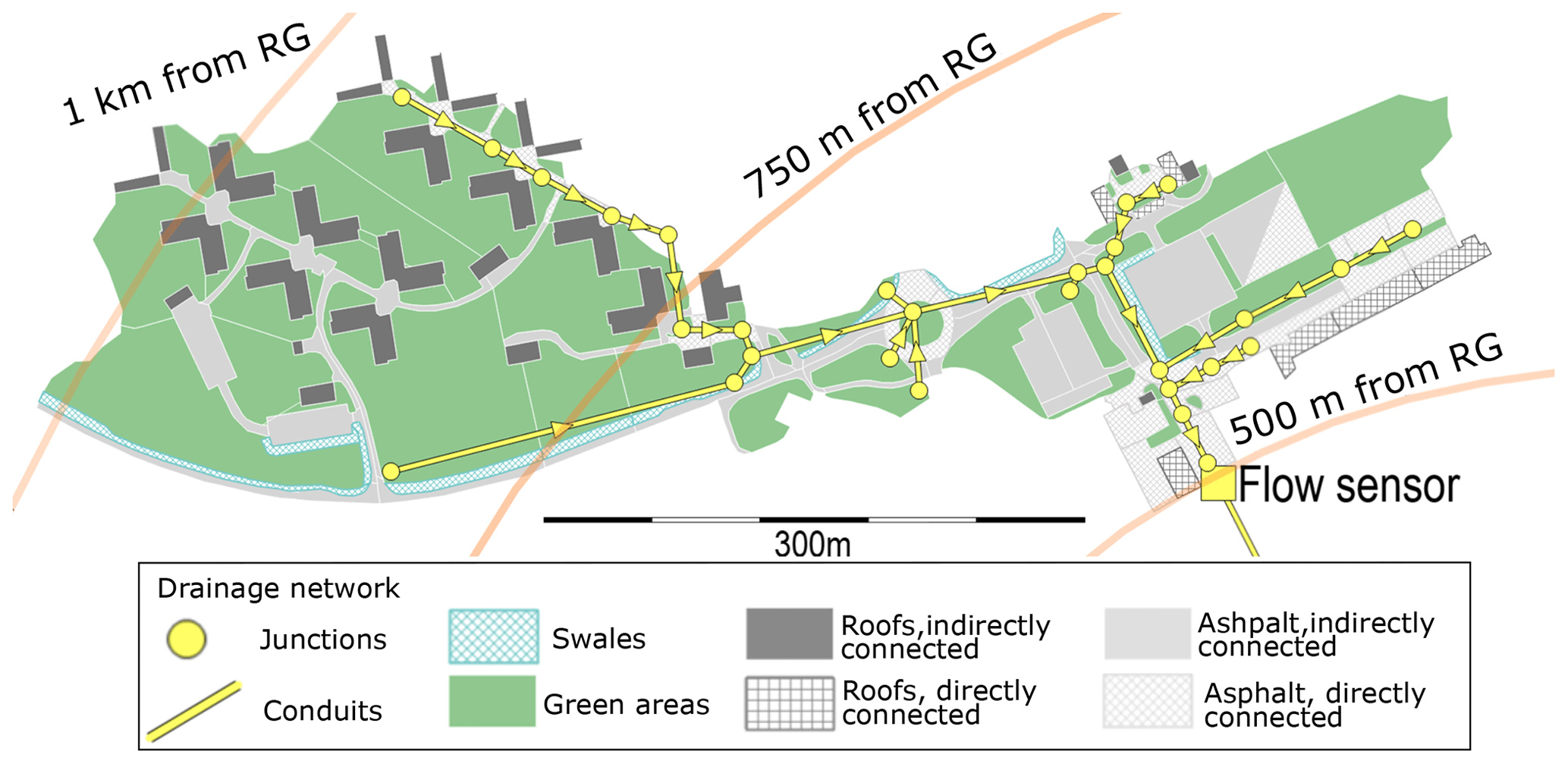
Figure 1Map of the studied catchment showing elements of the high-resolution rainfall–runoff model (see Sect. 2.2) and the distance of the catchment to the rain gauge (RG). The diameters of the pipes range from 400 mm for the main trunk where the flow sensor is located to 200 mm for the smaller branches.

Precipitation was measured at 1 min intervals with a Geonor T200B weighing-bucket precipitation gauge located outside of the study catchment, about 500 and 1000 m from the nearest and furthest borders of the catchment respectively (see circles in Fig. 1). The gauge was tested in the field and confirmed to work well twice a year in 2016 and 2017, and before 2016 such tests were also performed occasionally. Laboratory and field tests (by others) found this design of precipitation sensor to be a reliable instrument (Duchon, 2002; Lanza et al., 2010). Records were available for individual rain events in 2013–2015 and continuously for 2016 and 2017.

Flow rates in the storm sewer draining the catchment were measured at 1 min intervals by means of an ISCO 2150 AV (area velocity) sensor (a combination of an acoustic Doppler velocimeter and a pressure transducer) installed in the catchment outlet formed by a 400 mm diameter concrete sewer pipe. This type of sensor was assessed in the laboratory by Aguilar (2016) and found to have a combined uncertainty (consisting of bias, precision and benchmark uncertainty) of ±19.0 mm for the water depth measurements (the test range was 10–150 mm) and ±0.0985 m s⁻¹ for the velocity measurement (test range 0.1–0.6 m s⁻¹). These tests were carried out in a 0.46 m wide square channel, so the stage–discharge relationship was different from the study site described herein. It was also reported that the field performance of this type of sensors can suffer from the presence of too few (Teledyne ISCO, 2010) or too many particles suspended in the water (Nord et al., 2014).

While the difficulties in estimating all the uncertainties at the actual field site prevented a precise determination of the uncertainties’ magnitude, the general lab tests of the sensors used confirmed the acceptability of their records for the study purpose. Finally, it was also confirmed by Dotto et al. (2014) that errors in the calibration data can be compensated for in the calibration process.

The available precipitation record was divided into rainfall events with a minimum inter-event time of no precipitation of 6 h. Events deemed suitable for use in calibration were selected using the following criteria:

1. a minimum total precipitation of 2 mm (Hernebring, 2006);

2. no or small gaps in rain and flow data, i.e. both have to be available for > 90 % of the event duration;

3. sufficient in-pipe water depths for the flow sensor to work reliably: > 10 mm during at least 50 % of the event and > 25 mm at least once in the event, based on recommendations from the manufacturer (Teledyne ISCO, 2010);

4. peak flow > 2 L s⁻¹, since relative measurement uncertainties are high below this point;

5. no snowfall or -melt, since these would introduce additional processes in the hydrological behaviour and model of the catchment.

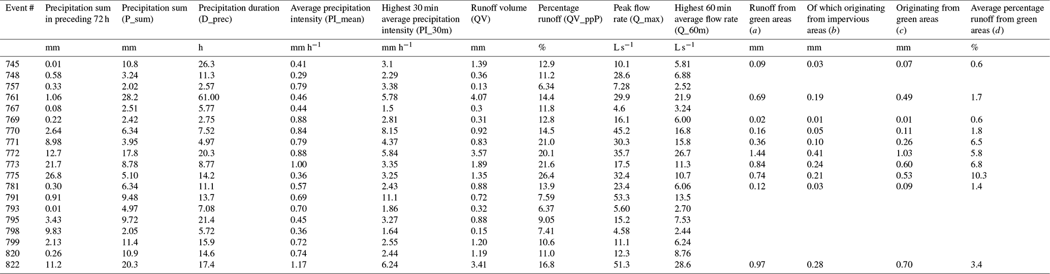
Calibration and validation periods were separated by using the 19 observed events from 2016 for the validation period and the 32 events from 2013–2015 and 2017 for the calibration period. In this way, all the calibration strategies (see Sect. 2.3) were tested (validated) against the same dataset, and no calibration strategies could benefit from including calibration events that also appeared in the validation set. The year 2016 was selected as the validation period for two reasons: it was the year with total precipitation closest to the annual mean, and the measured data records were continuous. Table 1 contains an overview of all events that were used in at least one calibration strategy as well as an initial estimate of the runoff from green areas.

Table 1Characteristics of all rainfall events used in one or more calibration strategies.

^a Calculated assuming 100 % runoff from impervious areas: a= QV – 0.12 P_sum, where 0.12 is the percentage of directly connected impervious area. (Some of this runoff originated from impervious areas that drained to green areas). ^b Calculated as $b=a(\mathrm{25}/(\mathrm{25}+\mathrm{63}\left)\right)$, where 25 and 63 are the percentages of indirectly connected impervious surfaces and green surfaces respectively. ^c Calculated as $c=a--b$. ^d Calculated as $d=c/$P_sum.

Download Print Version | Download XLSX

2.2 Runoff model and calibration approach

The US Environmental Protection Agency (EPA) Storm Water Management Model (SWMM) was selected, since it is a commonly used semi-distributed urban drainage model that allows to route runoff from one subcatchment to another. This routing feature was needed, since it allows for a high-resolution (HR) model setup in which each subcatchment (146 were used in total) features a single land cover. The high-resolution input data needed for this approach was available in the form of GIS data, aerial photographs and observations from site visits. The advantage of these single land-cover subcatchments is that their parameter values maintain their physical meaning and can be calibrated (or appropriate values found in the literature) for each land use or cover. Some spatial characteristics, such as the slope and the width of subcatchments, can be estimated more easily for smaller, uniform subcatchments. This approach has been used successfully by e.g. Krebs et al. (2014, 2016), Petrucci and Bonhomme (2014), and Sun et al. (2014). Within SWMM the Green-Ampt infiltration method was selected, since it can be calibrated with just two parameters (Rossman, 2016).

Whenever feasible, parameters for different subcatchments were set directly from the available GIS data and site visits, i.e. the sizes and slopes of all subcatchments and sewer pipes, as well as the catchment widths of small and disconnected roofs. For other subcatchments the catchment width was calibrated together with the other model parameters. To reduce the scope of the calibration problem, parameters were grouped based on land cover, yielding a total of 13 calibration parameters for the hydrodynamic model. Parameter values were limited based on values reported in the literature (see Table 2). To test whether the different calibration strategies showed different sensitivity to the model discretization, a low-resolution model (LR) setup was also used. Here each subcatchment was created by aggregating multiple smaller subcatchments from the high-resolution model. The area and percentage imperviousness of each aggregated subcatchment were calculated from its constituent smaller catchments. The calibration parameters were modified accordingly, as shown in Table 3, with the total number of calibration parameters being the same.

Table 2Calibration parameters and their ranges.

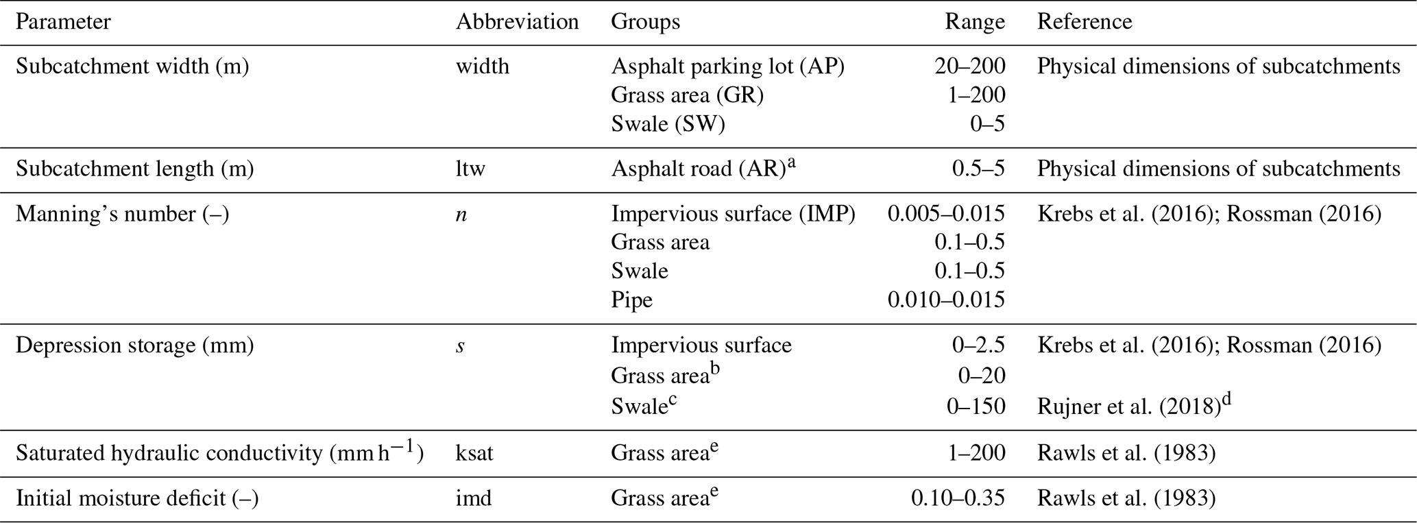
^a In SWMM, the subcatchment width is an input, but in this group of subcatchments, the length (in the flow direction) showed more similarity among the subcatchments, so it was calibrated instead of the width. ^b Includes vegetation and trees as well. ^c The maximum value was intentionally set high, since the swales' outlets are not always located exactly at the lowest points and the swales can be observed with larger ponds after heavy rain events. ^d Field experiments on similar swales in the same city. ^e Used for both grass areas and swales.

Download Print Version | Download XLSX

The precipitation gauge was situated a few hundred metres outside of the actual catchment and may have provided a biased estimate of the catchment rainfall. Therefore, a rainfall multiplier for each individual rainfall event was included in the calibration. This approach has been used with satisfactory results e.g. by Datta and Bolisetti (2016), Fuentes-Andino et al. (2017), and Vrugt et al. (2008), although it is limited by assuming a simple multiplicative difference between the gauge and catchment-average rainfall, which is not necessarily the case (Del Giudice et al., 2016). Furthermore, rainfall multipliers do not address the spatial variability of the rainfall, but in the absence of multiple rain gauges or other information about the spatial variability of rainfall in the study catchment, there were no feasible alternatives in this case. The rainfall multipliers create a way of adjusting the rainfall volume in the calibration so that the simulated runoff volume can better match the observed runoff volume. However, the multipliers do not allow distinguishing between (1) deviations between rainfall at the gauge and the catchment-averaged rainfall, (2) errors in the rainfall measurement, and (3) errors in the runoff measurement. A more traditional approach would be to calibrate the percentage of impervious areas, but in view of the availability of high-resolution land-cover information, it was preferred to apply rainfall multipliers instead.

Table 3Calibration parameters and their ranges for the low-resolution model.

^a For two subcatchments the percentage routed was estimated at 0 % and 100 % respectively. A single percentage was calibrated and shared by the three remaining subcatchments.

Download Print Version | Download XLSX

Green surfaces like those in the study area have a long hydrological memory for antecedent rainfall, and this had to be accounted for in the simulations. Neglecting this memory would increase the risk of green areas allowing unrealistically high infiltration in some rainfall events. Since SWMM does not allow for setting the initial values of state variables directly, such adjustments can be done by choosing an appropriate warm-up period for modelling runs. When sufficiently long warm-up periods are used, this approach offers an advantage consisting of treating the first rainfall–runoff peak of an event the same way as any following peaks, i.e. with initial conditions corresponding to a continuous simulation. The required length of this warm-up period was estimated by finding the last time before each rainfall event when the study area was dry. This was calculated for all rainfall events using the actual precipitation data and various values of the maximum depression storage and infiltration rate. The last antecedent time when the study area was dry was then used as the starting point of the warm-up period. This lookup procedure was applied to every event for each iteration in the calibration process so that all events were treated the same way as in a continuous simulation.

In the calibration process, the Shuffled Complex Evolution-University of Arizona algorithm (SCE-UA; Duan et al., 1994) was used to estimate the optimal values of the parameters. The algorithm was selected because it is commonly used in hydrological studies and allows for parallel computing. The Python library SPOTPY (Statistical Parameter Optimization Tool) (Houska et al., 2015), which includes this algorithm, was used to carry out the entire calibration process.

2.3 Event selection

This paper investigates single- and two-stage calibration strategies (CS), with each CS using six rainfall events. The single-stage CSs used the six events with the highest values for a given event characteristic and calibrated all parameters simultaneously. Two-stage calibration strategies calibrated first the parameters related to impervious areas, using a set of three rainfall events, followed by the pervious-area parameters using another set of three rainfall events. Since only 12 % of the total catchment surface is impervious and connected directly to storm sewers, it was assumed that the events, for which runoff volume was less than 12 % of rainfall volume, produced runoff only from impervious areas. Therefore, these events were suitable for calibration of impervious-area parameters in the first stage of the calibration process. It is conceivable that there is some contribution of green areas when the percentage runoff is less than 12 %. In that case the threshold should be set at a lower value, but since the amount of green-area runoff and the appropriate value of the threshold would be highly dependent on antecedent conditions, this was not included here. Following this step, events with more than 12 % runoff were assumed to also include runoff from green areas and were used to estimate pervious-area parameters in the second stage of the calibration. When calibrating the green-area parameters, the parameters related to impervious areas were kept fixed at their values from the first stage. This procedure splits the optimization problem into two smaller problems that have fewer parameters and shorter run times. The smaller number of parameters (reduced dimensionality) can ease the search for optimal parameter sets, while the shorter run time per iteration allows for a shortening of the total time needed, increasing the number of iterations used or including more events in the calibration.

Characteristics related to the rainfall, flow depths and flow rates were calculated for each event. For the single-stage calibration strategies, the six highest ranking events for each characteristic were selected. For the two-stage calibration strategies, the three highest ranking events with less than 12 % runoff were selected for the first stage and the three highest ranking events with more than 12 % runoff were selected for the second stage. Applying the calibrated rainfall multipliers in the calibration (Sect. 2.2) means that event properties relating to rainfall and percentage runoff will change, and the percentage of runoff can change from <12 % to >12 % and vice versa. Adjusting which calibration stage the events are available for in the calibration procedure (in a manner that is consistent for all events) would require (1) re-calculating which events should be available in each stage, (2) estimating in some way rainfall multipliers for all events, including those not initially selected by any calibration strategy, (3) re-calculating which events are used in each CS and (4) repeating the calibration for any CS that has had any of its events changed. Although this might improve the overall results of the proposed calibration procedure, it would also increase the complexity and raise several new issues, such as how to obtain a calibrated rainfall multiplier for the 10 events that were not used in any CS. We considered this to be beyond the paper’s original scope of examining different strategies for calibration event selection and proposing a practically useable two-stage calibration procedure.

To avoid making the comparison too large in scope, a limited number of calibration strategies (eight single-stage and six two-stage) was selected for use in this study. This selection was made so that it included a range of different characteristics and avoided multiple CSs with the exact same setup of events. The names of the CSs (see Table 4) consist of two or three elements:

• T6 (top 6) for single-stage or T32S (top 3–2 stages) for two-stage scenarios.

• The relevant event characteristic: precipitation (P), precipitation intensity (PI), runoff flow rate (Q), flow volume (QV), flow volume as percentage of rain QV_ppP or precipitation duration D_prec.

• The duration over which the characteristics were calculated: sum, mean and max refer to the whole event. Referring to the time interval used to calculate an average rainfall intensity or flow rate are the values 30 and 60 min (i.e. the highest value found within the event for a 30 or 60 min moving average). Calculating rainfall intensities and average flow rates over these windows rather than the entire event suppresses the effects of e.g. dry periods within events on such calculations.

The calibration strategy N_T6 consists of the six events that were selected most often in other calibration strategies with the goal of obtaining a set of events that score highly on a variety of characteristics.

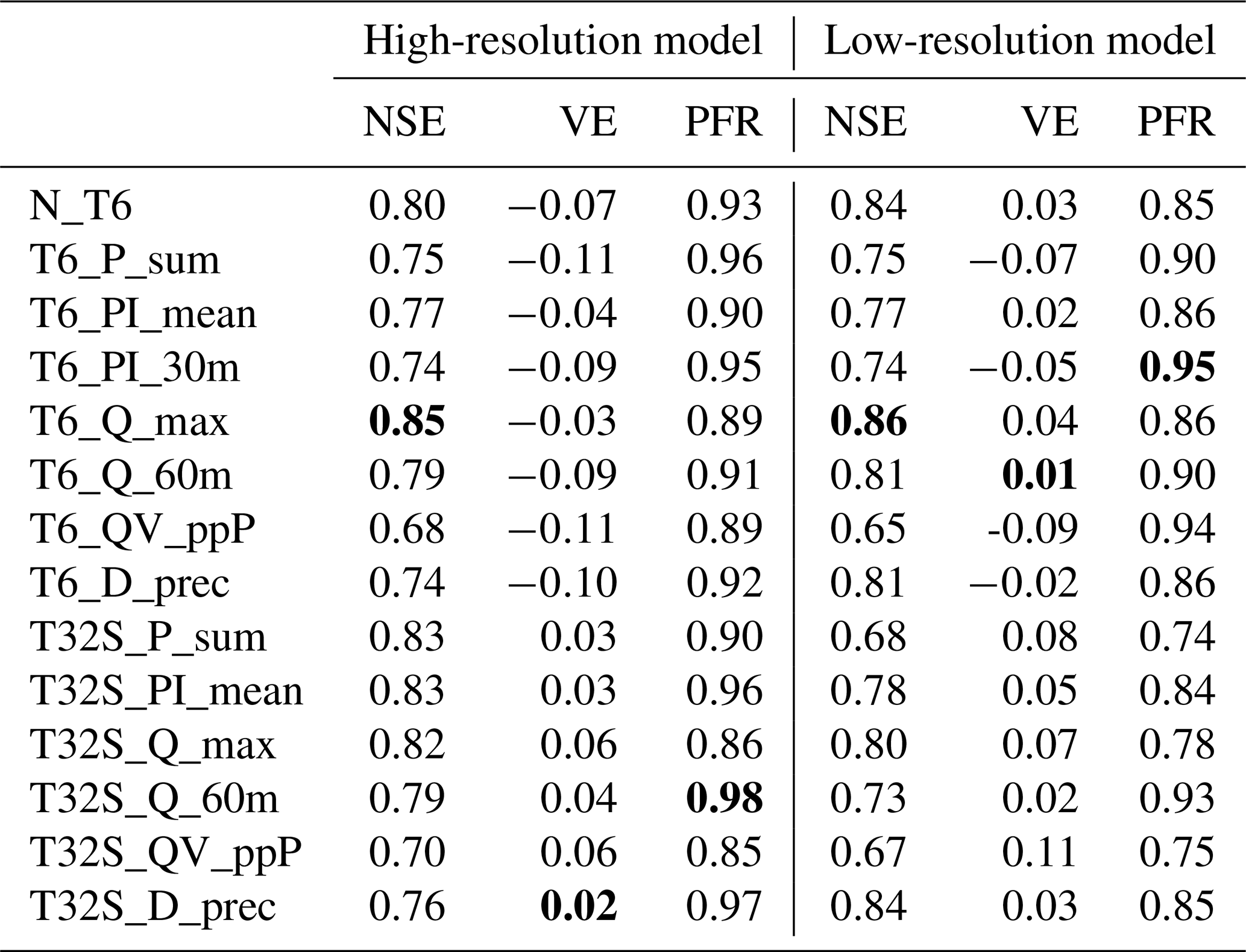
Table 4Calibration results. Bold font indicates the best value in each column.

Download Print Version | Download XLSX

2.4 Objective functions

The objective function used for the calibrations was the Nash–Sutcliffe efficiency (NSE):

where O denotes observed values and S denotes simulated values. The NSE measures the variance of the model errors (the numerator) as a fraction of the variance of the observations (the denominator). This fraction is then scaled so that it extends from negative infinity (i.e. the worst possible fit) via zero (the score that would be achieved by using the average of observations) to positive one for a perfect fit. The NSE is dimensionless, so it allows for comparing runoff events of different magnitudes. However, when the variance of the observations is small (e.g. for small runoff events), it can become quite sensitive to small changes in the simulated hydrograph. The NSE was calculated for each individual event and the mean over all events used as the calibration objective. For a further assessment of the modelled hydrographs, two metrics related to the peak flow and the hydrograph volume were used. The peak flow ratio (PFR) was defined as the ratio of the highest simulated to the highest observed flow rates, regardless of the times when they occurred.

where values >1 indicate overestimated simulated peak flows and values <1 indicate underestimated simulated peak flows. Finally, the relative volume error (VE) considers total flow volumes throughout the event.

It is positive when the simulated total flow volume exceeds the observed one and vice versa. Note that the above formula is only valid if the observation interval is constant. The peak flow ratio and volume error were used here since peak flow rates and storage volumes are often the targets that drainage systems are designed for.

The quick response of the studied catchment means that low-flow rates may cover a significant part of the event. Measurements in this range have relatively high uncertainties and may be considered less relevant than periods with higher flows. Therefore, it should be avoided that low flows dominate the analysis, which was achieved by including only time steps with observed flow rates >1 L s⁻¹ in calculating these metrics.

3.1 Calibration performance

The high-resolution model was successfully calibrated for all calibration strategies, with an event mean NSE for all events ranging from 0.68 to 0.85 (see Table 4). The lowest event mean NSE corresponded to the two CSs based on the percentage runoff (T6_QV_ppP and T32S_QV_ppP). This result can be attributed to one event (see Fig. 2b), for which both CSs resulted in simulated hydrographs with a low NSE, in spite of a visually good fit of the observed data. In this case, a low NSE resulted from a small timing error and from low-flow rates in the event, which led to a low variance of the observations and, therefore, an NSE that is more sensitive to small simulation errors. For the two-stage calibration strategies, the individual stages also produced successful calibrations (stage 1 event mean NSE of 0.70–0.87; stage 2 event mean NSE of 0.78–0.87), except for the second stage in T32S_QV_ppP for the reasons explained above. The NSE values for the individual calibration events in the different calibration strategies are similar to those reported by Krebs et al. (2013). Using the HR model, there were four event characteristics (P_sum, PI_mean, QV_ppP and D_prec) for which the two-stage calibration performed better (up to 0.08 event mean NSE) than the single-stage calibration, while for Q_max the single-stage calibration performed better (0.03 event mean NSE). However, when using the low-resolution model, three event characteristics (P_sum, Q_max and Q_60m) had better performance with the single-stage than with the two-stage approach. Overall, N_T6, T6_Q_max and T32S_Q_max performed best (being the only CSs with an event mean NSE >0.8 in both the HR and LR models), while the two scenarios based on percentage runoff performed worst.

Figure 2Examples of hydrographs for events with high (a) and low (b) objective function (NSE) values; var_obs denotes the variance of the observations.

Download

Considering the errors in total runoff volume, the two-stage CSs performed better for the HR model. However, for the LR model (where runoff volumes were higher in general, as also reported by Tscheikner-Gratl et al., 2016), the single-stage calibrations had smaller volume errors. The changes in volume errors between the HR and LR model were similar to earlier findings by Krebs et al. (2016). Although the CSs based on peak flow rates (Q_max) performed well in terms of the event mean NSE, they are actually among the worst performers in terms of peak flow ratio in both the HR and LR model. This may be attributed to the possibility for models to obtain high NSE values despite underestimating high peak flows (see Fig. 2a). In general the LR model resulted in lower peak flow ratios (as also shown by Tscheikner-Gratl et al., 2016), and this effect was stronger for the two-stage CSs.

For the two-stage calibrations the assumption that no runoff occurred from green areas during the first stage of the calibration was checked. During the actual first-stage calibration (i.e. with green-area parameters set to default values) there was no runoff from green areas for any of the calibration events in any of the calibration strategies, so the first-stage calibration attributed all runoff to impervious areas as assumed beforehand. However, some runoff occurred from green areas for first-stage events when the calibrated parameter values from the second stage were applied. This runoff was caused by impervious areas draining to green areas. The runoff from green areas was <5 % of the total simulated runoff volume for four model runs, <10 % for an additional three runs, and 11.6 %, 11.7 %, 21.7 %, 22.9 % and 25.7 % respectively for five additional runs. Note that with six CSs with three first-stage events each, there were 18 model runs in total. The last mentioned five runs concerned three different events with a percentage runoff (calculated before applying rainfall multipliers) between 11 % and 12 %. Such events may be expected to include some green-area runoff, and it could be considered to exclude these from the first-stage calibration (not done here to limit the complexity of the procedure as discussed in Sect. 2.3). In addition, all three events were also included in other first-stage calibrations where they did not result in any significant simulated green-area runoff. Removing these events from the first stage of calibration based on initial calibration results would therefore result in the same event being included in different stages for different calibration strategies, which was considered undesirable. Overall we believe that, although the assumption that all runoff is from directly connected impervious areas when QV_ppP <12 % is violated in some cases, the assumption that these events are suitable for calibrating impervious-area parameters does hold to a sufficient degree, as also evidenced by the good first-stage calibration performance (see first paragraph of this subsection). In addition, checking for green-area runoff as done here is only possible after calibration, and considering it when selecting events would thus create a more complex, iterative calibration procedure, which would limit the practical applicability of this approach. We considered this to be beyond the paper's original scope of examining different strategies for calibration event selection.

3.2 Calibrated parameter values

3.2.1 Hydrologic model parameters

Figure 3 shows the calibrated parameter values (for the HR model), normalized with respect to their calibration ranges (see Table 2). There is considerable variation among the calibrated values obtained in different calibration strategies, demonstrating that even for parameters with a clear physical interpretation, identification of the best (ideal) value is not straightforward. Gupta et al. (1998) also found considerable variation in the parameter values obtained when using different years as calibration periods for a natural catchment model. Nonetheless, the span of parameter values is considerably reduced compared to the range imposed during calibration, showing that the boundaries were not set too tightly and that the calibration procedure does offer benefits over estimating parameter values directly. The variation among the two-stage CSs was larger than that among the single-stage CSs for most parameters, which may be caused by the dataset used to estimate each parameter being smaller (three events instead of six). The depression storage in green areas and swales might be compensating for each other in the two-stage CSs. The depression storage for impervious areas shows little variation (0–0.3 mm) between the different CSs, with only T6_Q_60m resulting in a slightly higher value (0.5 mm).

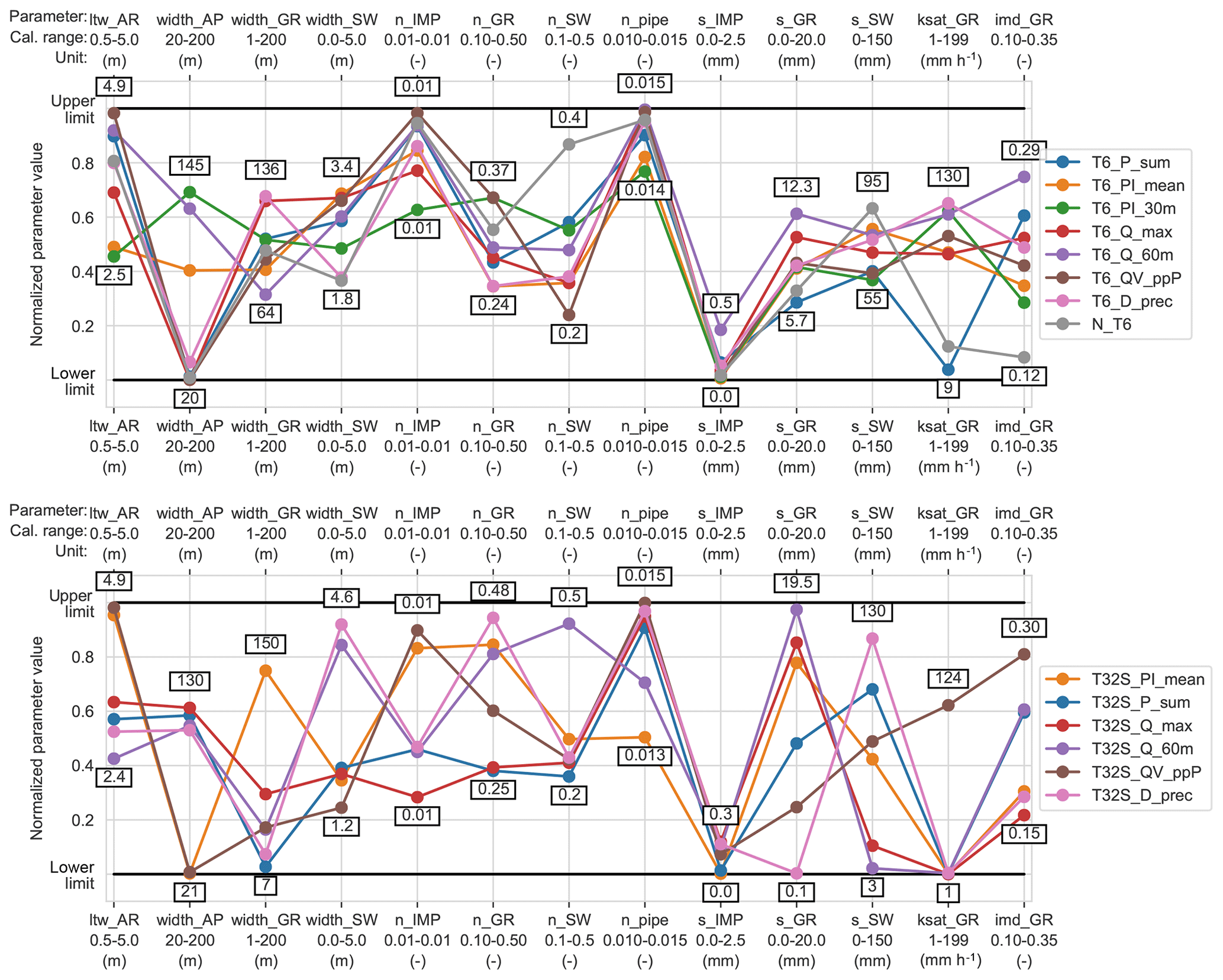
Figure 3Normalized calibrated parameter values for the high-resolution model using different calibration strategies. The highest and lowest values found for each parameter are indicated.

Download

Calibrated parameter values are always uncertain estimates. This uncertainty has been investigated for urban drainage models and shown to be dependent on parameter type, study catchments, model structures, catchment discretization and measurement errors (Dotto et al., 2009, 2011, 2014; Kleidorfer et al., 2009a; Sun et al., 2014). The variation found here among the optimum parameter values obtained in different calibration strategies suggests that the selection of calibration events could also affect the uncertainty of parameter estimates, and this influence should be investigated further.

3.2.2 Rainfall multipliers

The values of rainfall multipliers found in the calibration process ranged from 0.48 to 2.92, indicating a mismatch between the observed rainfall and the rainfall that allows for the best fit of the simulated runoff to observed runoff. Several factors may contribute to this. First, an underestimation of rainfall or underestimation of runoff by the respective sensors may lead to higher rainfall multipliers and vice versa. Errors in the size of (sub-)catchments may also influence this. Second, the gauge rainfall may not match the catchment-averaged rainfall due to the spatial variability of the rainfall. Thirdly, some deficiencies in the model may be compensated for, to some extent, by adjusting the rainfall multiplier. Without further investigations it is not possible to distinguish between different factors influencing the values of rainfall multipliers. Two arguments support that the rainfall multipliers do indeed fulfil the role of compensating for this mismatch. Firstly, for rainfall events that were included in multiple calibration strategies, the calibrated multipliers from different scenarios were close to each other (see Table 5), unlike for the hydrological model parameters (see Sect. 3.2.1). Secondly, decreasing or increasing all flow rates by 40 % prior to calibration changed the average rainfall multipliers by −37 % and +33 % respectively. The average value of the rainfall multipliers across all events was 1.2, which suggests that there was some structural disagreement between the observed rainfall and flows. The close agreement between the different CSs shows that, unlike the hydrological model parameters, the rainfall multipliers are not sensitive to differences between the CSs.

Table 5Calibrated rainfall multipliers (HR model) for all rainfall events that were used in at least one CS.

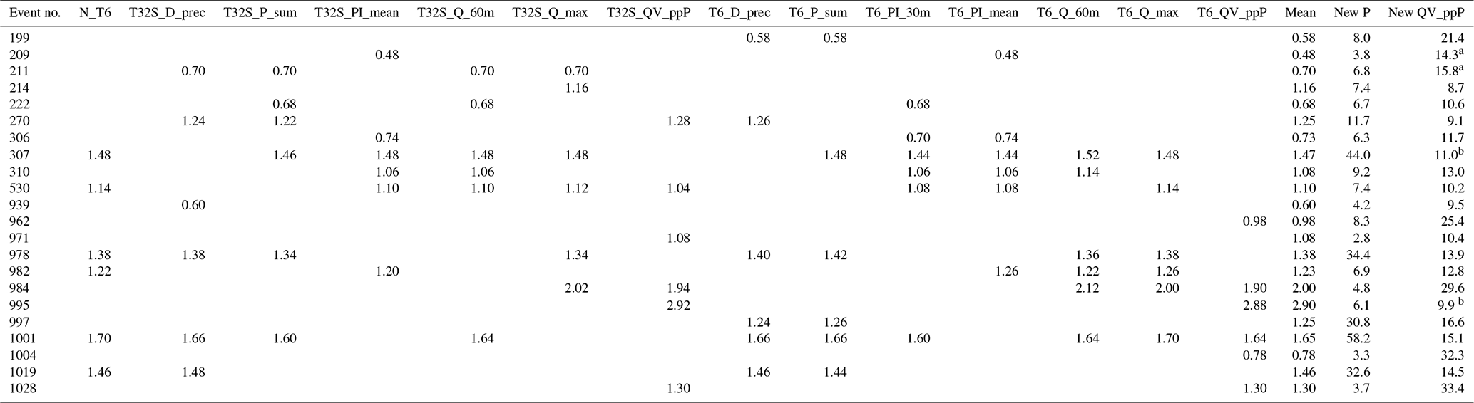
^a Event percentage runoff switches from <12 % to >12 % when applying the rainfall multiplier. ^b Vice versa.

Download Print Version | Download XLSX

3.3 Validation performance

3.3.1 Individual events

The validation performance for individual events is visualized in Fig. 4 for the peak flow ratio, volume error and NSE. The events that most often caused failure in validation were four events with peak flow rates of 10 L s⁻¹ or less (i.e. events 1–4 in the figure), and therefore, such failures may be attributed to (1) relatively high measurement uncertainties and (2) low variance of the observations leading to high sensitivity of the NSE to even small differences between observed and predicted hydrographs (see Sect. 2.4 and Fig. 2). However, it should be noted that the two smallest events (both with a peak flow rate of 4.6 L s⁻¹) were predicted with an NSE >0.5 by T6_P_sum and T32S_QV_ppP. For the other CSs, examination of the hydrographs showed that they predicted well the peak flow and the total runoff volume of the events, but they produced wrong timing compared to the observed hydrograph. Another event that failed in validation for all CSs was that with the highest peak flow rate (53 L s⁻¹; event 19 in Fig. 4, see Appendix A), which was overestimated by a factor of up to three. This event was dominated by an intense, single-peak burst of rainfall (the highest 30 min average rainfall intensity was 11.1 mm h⁻¹), so it could have suffered from high spatial variation of the rainfall.

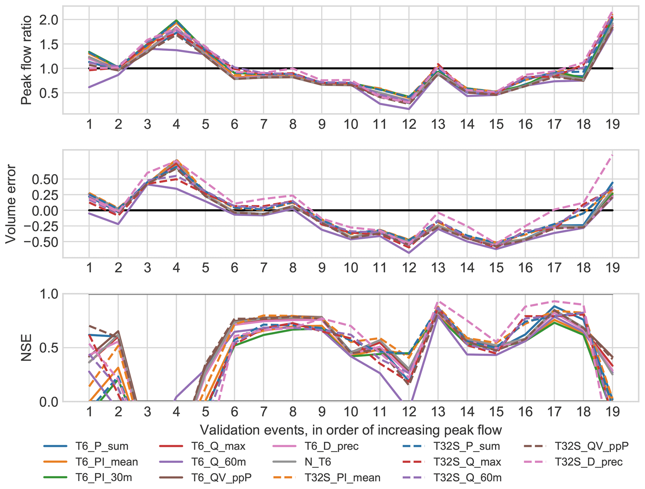
Figure 4Error statistics for individual validation events for all calibration strategies in the HR model.

Download

The peak flow ratios obtained for the 19 validation events using the calibrated high-resolution models are shown in the upper panel of Fig. 4. The under- or overestimation of peak flows and runoff volumes by the model could lead to an under- or over-dimensioned system design, and it is therefore relevant to consider these aspects alongside the NSE. The underestimation of peak flows was most frequent, but the largest errors occurred when the flow was overestimated. The variation among CSs was generally larger when the prediction error was larger. The corresponding figure for volume errors is shown in the middle panel of Fig. 4. Again, underestimation was more common, but overestimation did occur for a limited number of events. For both peak flows and total volumes, the variation among events was generally larger than the variation among different calibration strategies, showing that selecting a limited number of validation events may also influence the results of the model evaluation. T32S_D_prec stood out by predicting higher runoff volumes and peaks, and therefore better performance, for the events labelled 13–18 in Fig. 4. Across all CSs, two-stage versions had similar or better performance in terms of total runoff volume. Peak flow was underestimated for most events, but for the events that generally did poorly in validation (see above) peak flows (as well as flow volumes) were overpredicted instead. The results for both total volumes and peak flows indicate that for most events flows were underestimated, which may be (at least partially) attributed to the need to multiply the observed rainfall by (on average) a factor of 1.2 to best match the observed flow during the calibration phase (see Sect. 3.2.2); such an adjustment was not applied in the validation phase.

When examining the NSE of the validation events (see the bottom panel of Fig. 4), more variation among the different CSs became visible, although the amount of variation was still event-dependent: the difference (in NSE) between the best and worst CS for the same events varied from 0.15 to 1.25. This shows that some events can have a much larger impact on the overall validation results than others. Out of the 19 events, six were predicted satisfactorily (NSE >0.5) by some CSs but not by others; five events failed for all CSs; and eight were predicted satisfactorily by all CSs. For several events (10, 16 and 18) the two-stage CSs (except T32S_QV_ppP) showed better performance than the single-stage CSs, but there were no events where all the single-stage CSs performed better.

3.3.2 Overall performance

The successful CSs predicted 8–13 out of the 19 validation events satisfactorily (NSE >0.5) (see Table 6). T6_PI_30m (nine events) and T6_Q_60m (eight events) performed worst, while T32S_PI_mean performed best. For the single-stage CSs the low-resolution model predicted up to five fewer events satisfactorily than the high-resolution model, while from the two-stage CSs only T32S_D_prec satisfactorily predicted fewer events with the LR model than with the HR model, and T32S_P_sum, T32S_Q_max and T32S_QV_ppP actually predicted more events satisfactorily with the HR model.

Table 6Summarized validation performance (over 19 events) for the high-resolution model. Bold font indicates the best value in each column.

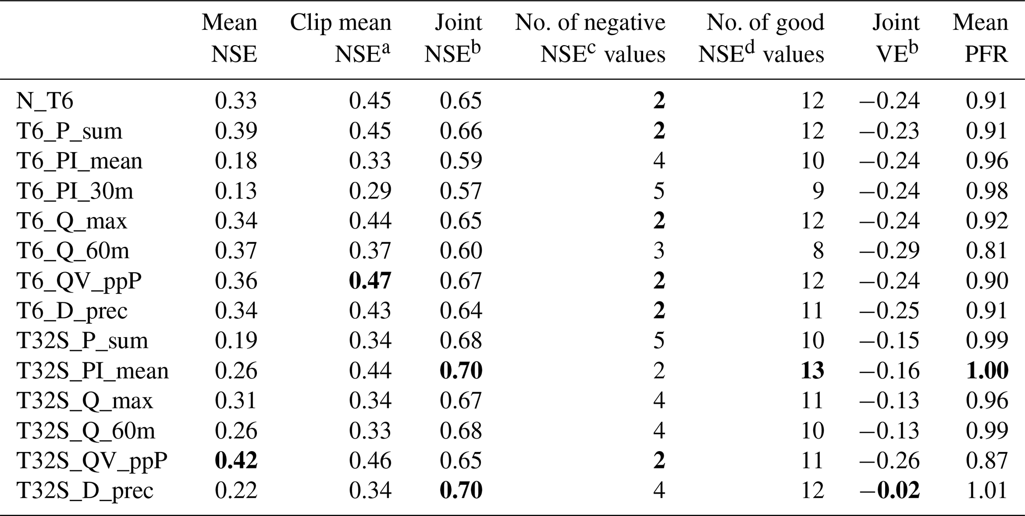
^a Calculated after setting individual event values $<-\mathrm{1}$ to −1. ^b Calculated after merging all event time series into a single series. ^c Number of events with an NSE <0. ^d Number of events with an NSE >0.5.

Download Print Version | Download XLSX

To assess the overall performance of different calibration strategies for the validation period, several ways of combining the individual events were considered (see Table 6). The simplest metric is obtained by using the NSE means, which ranged from 0.13 (T6_PI_30m) to 0.42 (T32S_QV_ppP). There are two conceptual problems with this metric. First, since the NSE ranges from negative infinity to positive one, one poorly fitting event can offset multiple well-fitting events. Second, two simulated hydrographs of an equally poor fit can have rather different (negative) NSE values, producing different impacts on the overall results, which is not justified by a visual comparison. Therefore, this mean metric is not considered a reliable metric for comparisons when poorly fitting events are present. The exclusion of low-flow (<10 L s⁻¹ peak) events would avoid this issue, but it would not reward calibration strategies that do manage to predict these events satisfactorily. Another option is to set all NSE values $<-\mathrm{1}$ to −1 before calculating the mean, which results in a mean NSE ranging from 0.29 (T6_PI_30m) to 0.47 (T6_QV_ppP). The two-stage CSs had worse performance than the single-stage CSs (except for PI_mean). A more commonly used approach is to combine all the events into a single time series prior to calculating the NSE on the joint time series. This procedure indicated satisfactory performance for all CSs with the NSE ranging from 0.57 (T6_PI_30m) to 0.70 (T32S_PI_mean and T32S_D_prec). This last metric also showed better performance for two-stage CSs than their single-stage counterparts (except for QV_ppP), i.e. the opposite of what was found for the mean NSE. The downside of this metric is that it can hide the fact that poorly fitting events are present, e.g. T32S_P_sum has the (shared) third-highest joint NSE, despite having five events with a negative NSE. The discussion of various metrics shows that caution is needed when averaging performance over multiple events, as metrics may not reflect the fact that a significant number of events is poorly predicted in all CSs. It depended on the chosen criterion as to which CSs performed best, but T6_PI_mean, T6_PI_30m and T6_Q_60m were always near the bottom in the NSE-based metrics and would therefore not be recommended. Of the two-stage CSs, T32S_PI_mean showed the best performance in the NSE-based metrics.

The considerations in the previous paragraph concern the NSE and are not necessarily applicable to other statistics in the same way. The volume error was included in this study to yield some indication of the overall difference between the modelled and observed runoff volumes over longer time periods. Therefore, this statistic was summarized over all events using the joint-time-series approach. The volume errors were similar for all high-resolution single-stage calibrated models and showed a general tendency to underestimate flow volumes by 25 %. For the two-stage calibrated models, volume errors were smaller with an underestimation of around 15 % (except for T32S_QV_ppP), and T32S_D_prec showed a volume error of only −2 %. The average peak flow ratio over all events indicated better performance for the two-stage CSs than for the single-stage CSs. The CSs based on rainfall intensity showed the best performance in terms of peak flows. T6_Q_60m had the worst performance for total volume and peak flow (despite being calibrated to events that score highly on both characteristics) and would therefore not be recommended.

For most of the LR model, two-stage calibrations had a higher event mean NSE than their single-stage counterparts (except for Q_max and Q_60m; see Table 7), and a visual comparison of the hydrographs showed that for most events the HR model performed better. However, the two-stage calibrations performed significantly better than their single-stage counterparts in terms of volume error and peak flow (see Table 7), and the two-stage CSs that were based on observed flow rates (T32S_Q_max and T32S_Q_60m) outperformed the HR model in the visual comparison of hydrographs.

Table 7Summarized validation performance (over 19 events) for the low-resolution model. Bold font indicates the best value in each column. The columns marked with ^* are not discussed in the text, but they are shown here for completeness and comparability with Table 6.

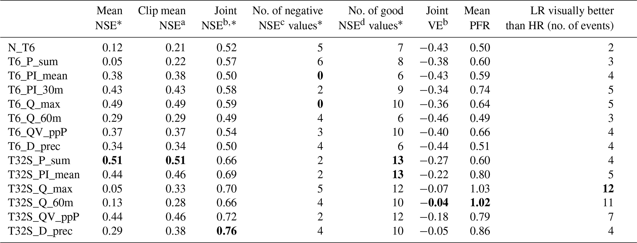
^a Calculated after setting individual event values $<-\mathrm{1}$ to −1. ^b Calculated after merging all event time series into a single series. ^c Number of events with an NSE <0. ^d Number of events with an NSE >0.5.

Download Print Version | Download XLSX

Figure 5Loss of performance (NSE) when switching from calibration to validation.

Download

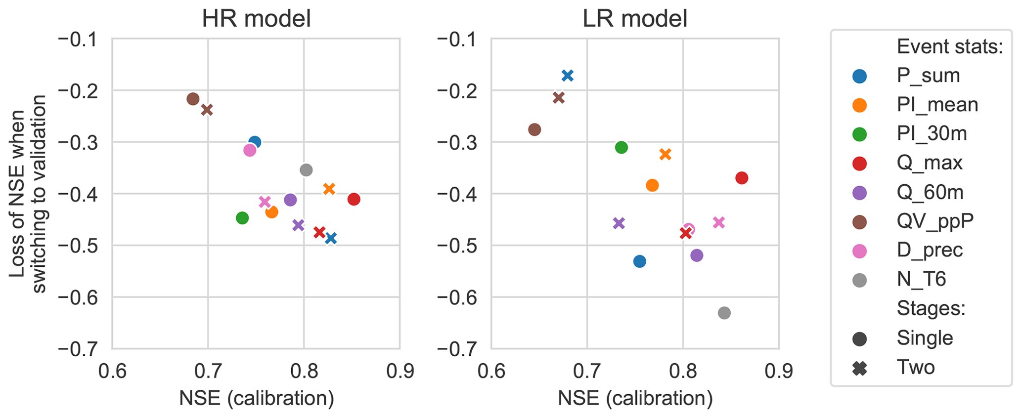
3.4 Degradation of performance from calibration to validation

In calibration, the event mean NSE for the different calibration strategies ranged (for the HR model) from 0.68 to 0.85, while in validation this was lowered to 0.29 to 0.47 (NSE values $<-\mathrm{1}$ were set to −1 prior to taking the mean; see Sect. 3.3.2). For the LR model the variation between different CSs was slightly larger, ranging from 0.65 to 0.86 in calibration and from 0.21 to 0.51 in validation. The CSs that did better in calibration lost more performance (measured by event mean NSE) when switching to the validation phase (see Fig. 5). In particular, the CSs based on percentage runoff (QV_ppP) had the worst calibration performance (in both HR and LR models) but lost the least when switching to the validation phase. For the high-resolution model all but one of the two-stage calibrations lost more performance when switching to the validation phase than their single-stage counterparts. By contrast, for the low-resolution model all but one of the two stage calibrations had a smaller performance loss. Previous studies found that high-resolution models led to more transferable parameter estimates (e.g. less loss of performance when switching to validation; Sun et al., 2014; Krebs et al., 2014), but in the current study this seems dependent on the calibration dataset used.

Figure 6Comparison of single-stage and two-stage calibration strategies.

Download

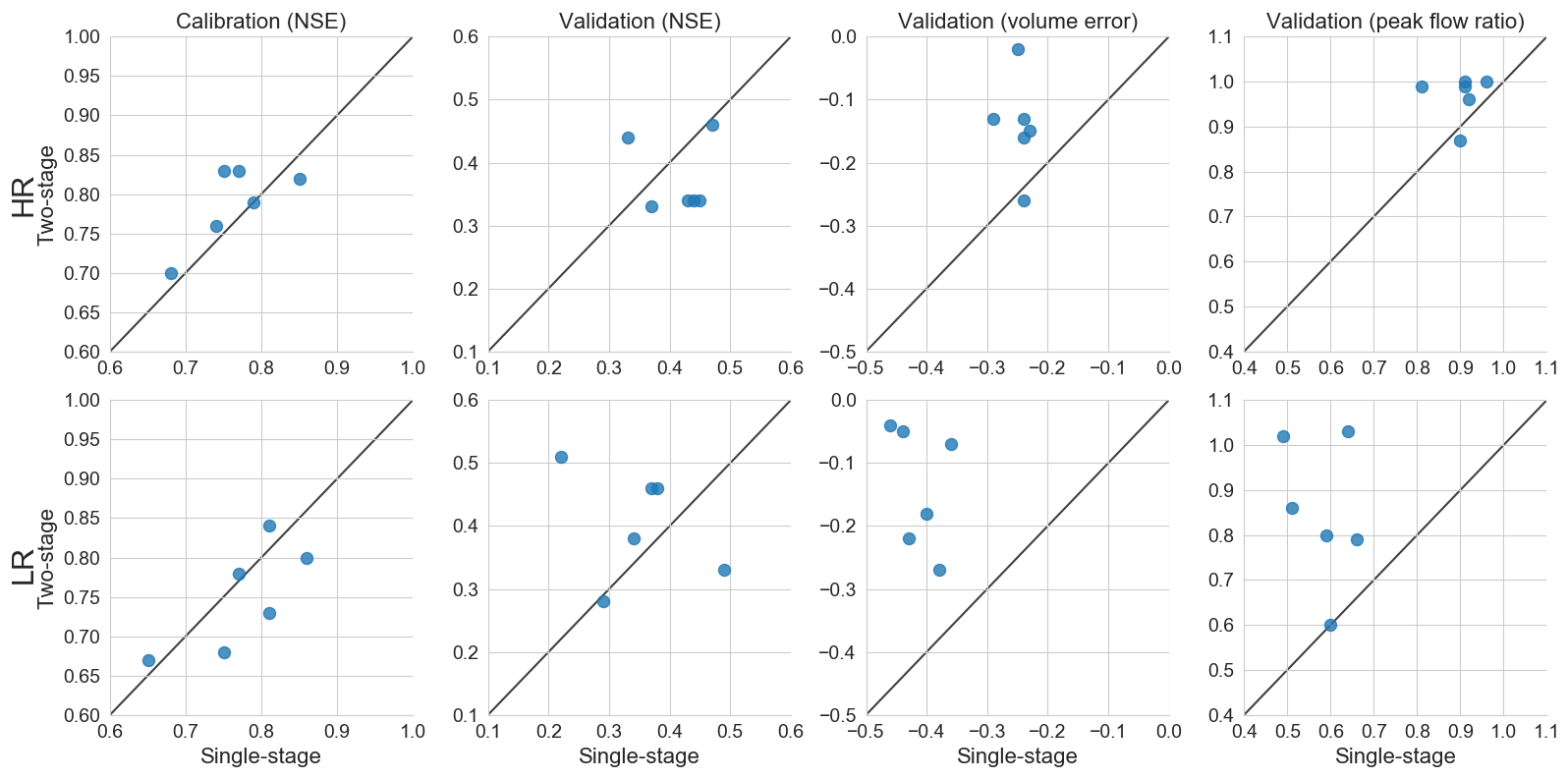
3.5 Single-stage vs. two-stage calibrations

For those selection criteria, for which both single- and two-stage calibrations were performed, the results of the two options can be compared directly (see Fig. 6). For the high-resolution model, calibration performance of the two-stage CSs was somewhat better than for the single-stage CSs. By contrast, in the validation phase the event mean NSE was better for the single-stage CSs. However, the volume error and peak flow ratio were better for the two-stage calibrations. For the low-resolution model performance was similar or worse for the two-stage calibrations, but in the validation phase the two-stage calibrations most often had a higher event mean NSE. In addition, the two-stage calibrations resulted in much better performance in terms of volume error and peak flows than their single-stage counterparts.